Diffusion Models Encode the Intrinsic Dimension of Data Manifolds
Overview
In this work, we theoretically and experimentally prove that diffusion models, extensively used in generative modeling, capture the intrinsic dimension of the data. We introduce a novel method for estimating this intrinsic dimension directly from a trained diffusion model.
Problem Setup
We consider the following setup:
- There is a data manifold \( \mathcal{M} \) of intrinsic dimension \( k \), embedded in an ambient Euclidean space \( \mathbb{R}^d \), where \( d \gg k \).
- There is a probability distribution \( p \) that is highly concentrated around \( \mathcal{M} \).
- We are given a finite sample of data \( \{ x_i \}_{i=1}^n \subseteq \mathbb{R}^d \) generated from \( p \).
Diffusion Models and the Score Function
We consider an Itô diffusion:
The time-reversed stochastic differential equation (SDE) is:
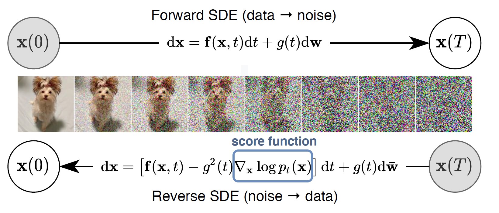
Figure: Forward and reverse SDEs
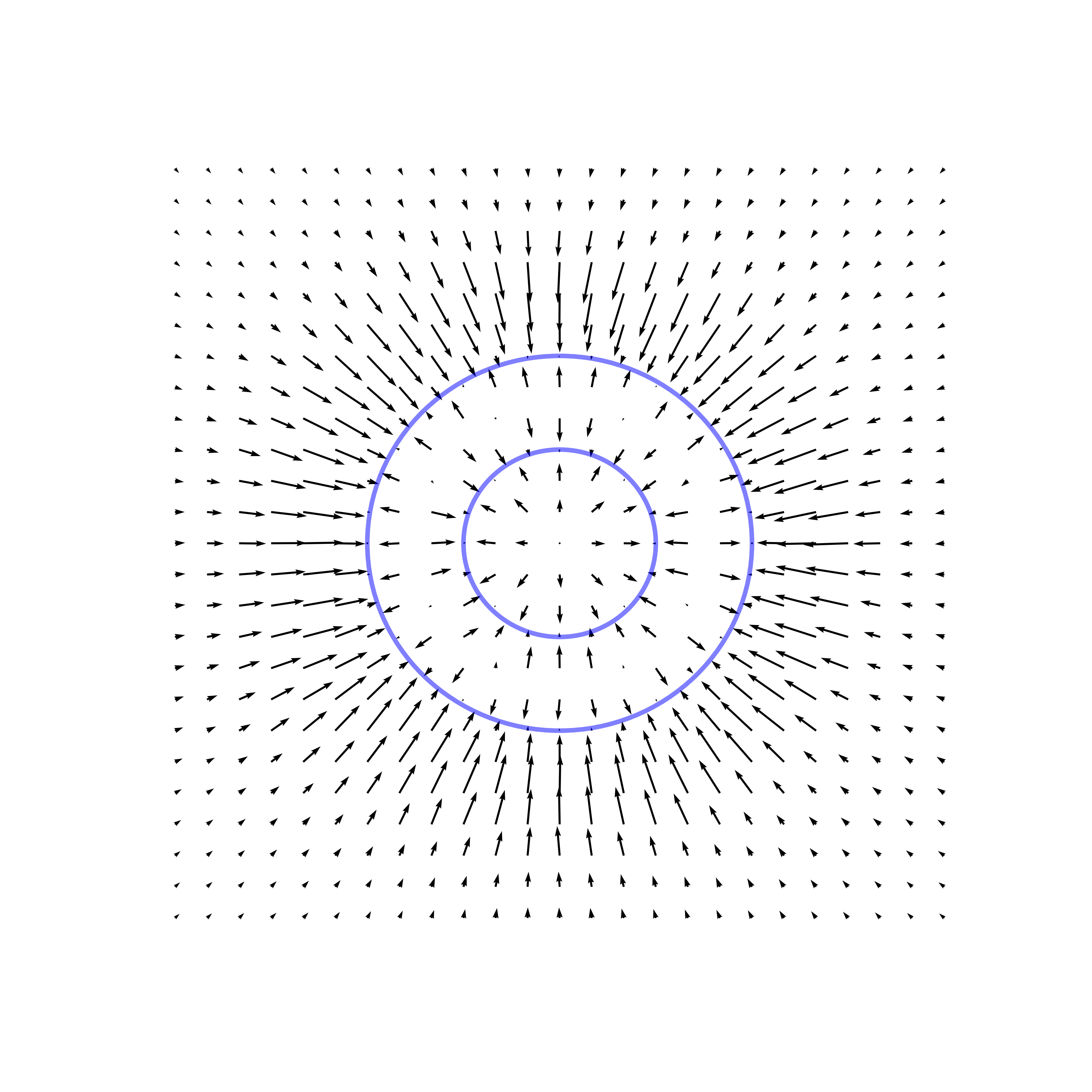
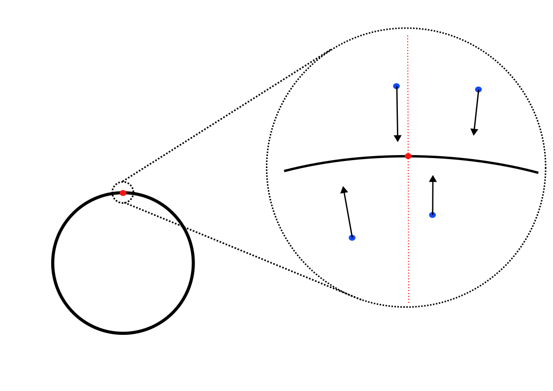
Key Observation: Score Field Perpendicular to the Manifold
To formalize this observation, let \( \pi(x) \) denote the projection of the point \( x \) onto \( \mathcal{M} \), \( \mathcal{N}_{\pi(x)}\mathcal{M} \) denote the normal space and \( \mathcal{T}_{\pi(x)}\mathcal{M} \) denote the tangent space of \( \mathcal{M} \) at \( \pi(x) \). The score vector \( \nabla_x \ln p_{\varepsilon}(x) \) predominantly lies within the normal space \( \mathcal{N}_{\pi(x)}\mathcal{M} \). Mathematically, this means that its projection onto the normal space is significantly larger than its projection onto the tangent space: \[ \left\| \text{Proj}_{\mathcal{N}_{\pi(x)}\mathcal{M}} \left[ \nabla_x \ln p_{\varepsilon}(x) \right] \right\| \gg \left\| \text{Proj}_{\mathcal{T}_{\pi(x)}\mathcal{M}} \left[ \nabla_x \ln p_{\varepsilon}(x) \right] \right\|. \] This phenomenon occurs because, at small \( \varepsilon \), the probability density \( p_{\varepsilon}(x) \) is sharply concentrated around \( \mathcal{M} \). The variations in \( p_{\varepsilon}(x) \) are much more pronounced in the normal direction than in the tangent direction, causing the gradient \( \nabla_x \ln p_{\varepsilon}(x) \) to point primarily towards \( \mathcal{M} \) along the normal.


Intrinsic Dimension Estimation Method
- \( s_\theta \): trained diffusion model (score function)
- \( t_0 \): small sampling time
- \( K \): number of perturbed points
- Sample \( \mathbf{x}_0 \) from the dataset \( p_0(\mathbf{x}) \).
- Set \( d = \text{dim}(\mathbf{x}_0) \).
- Initialize an empty matrix \( S \).
- For \( i = 1, \dots, K \):
- Sample \( \mathbf{x}_{t_0}^{(i)} \sim \mathcal{N}(\mathbf{x}_0, \sigma_{t_0}^2 \mathbf{I}) \).
- Append \( s_\theta(\mathbf{x}_{t_0}^{(i)}, t_0) \) as a new column to \( S \).
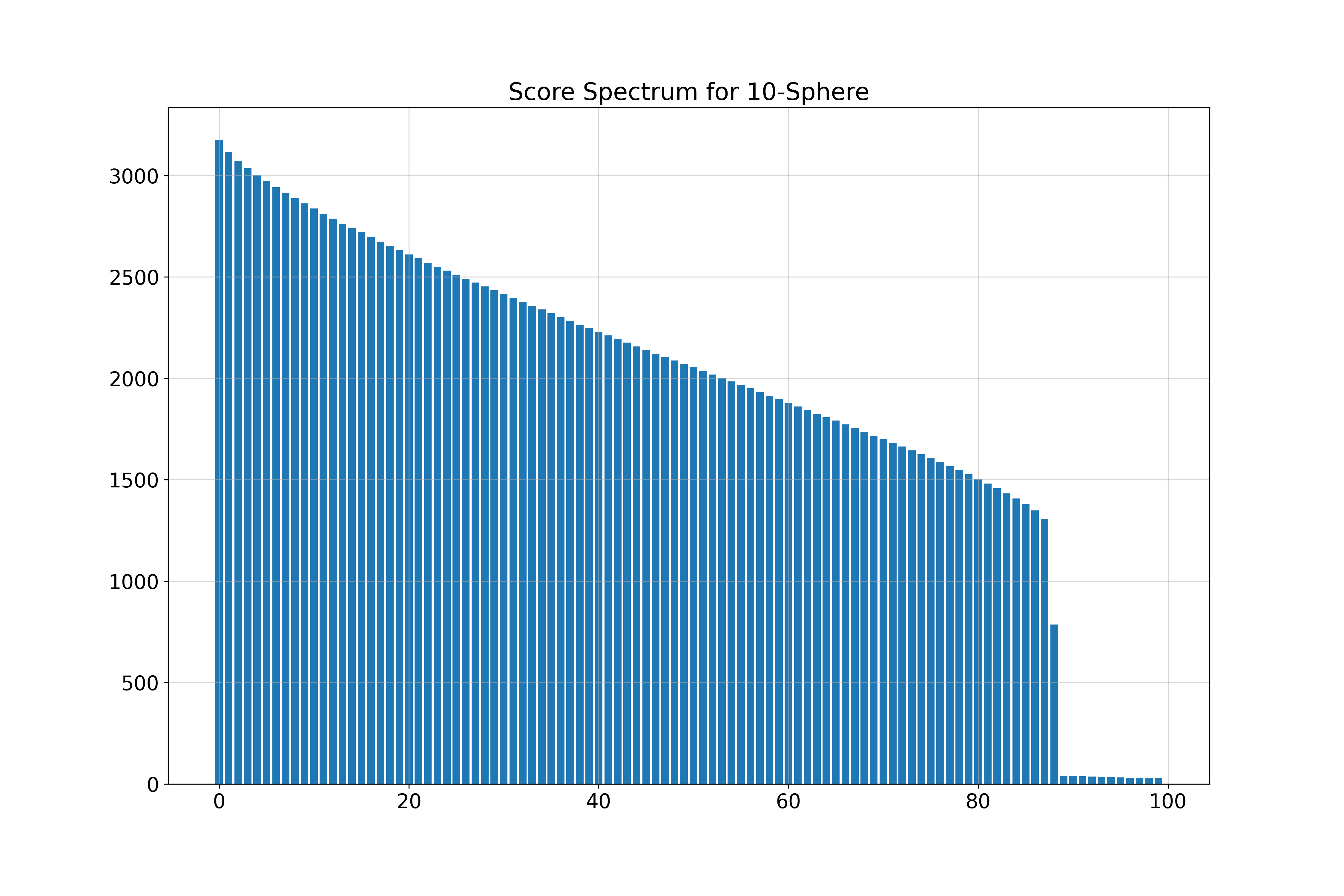
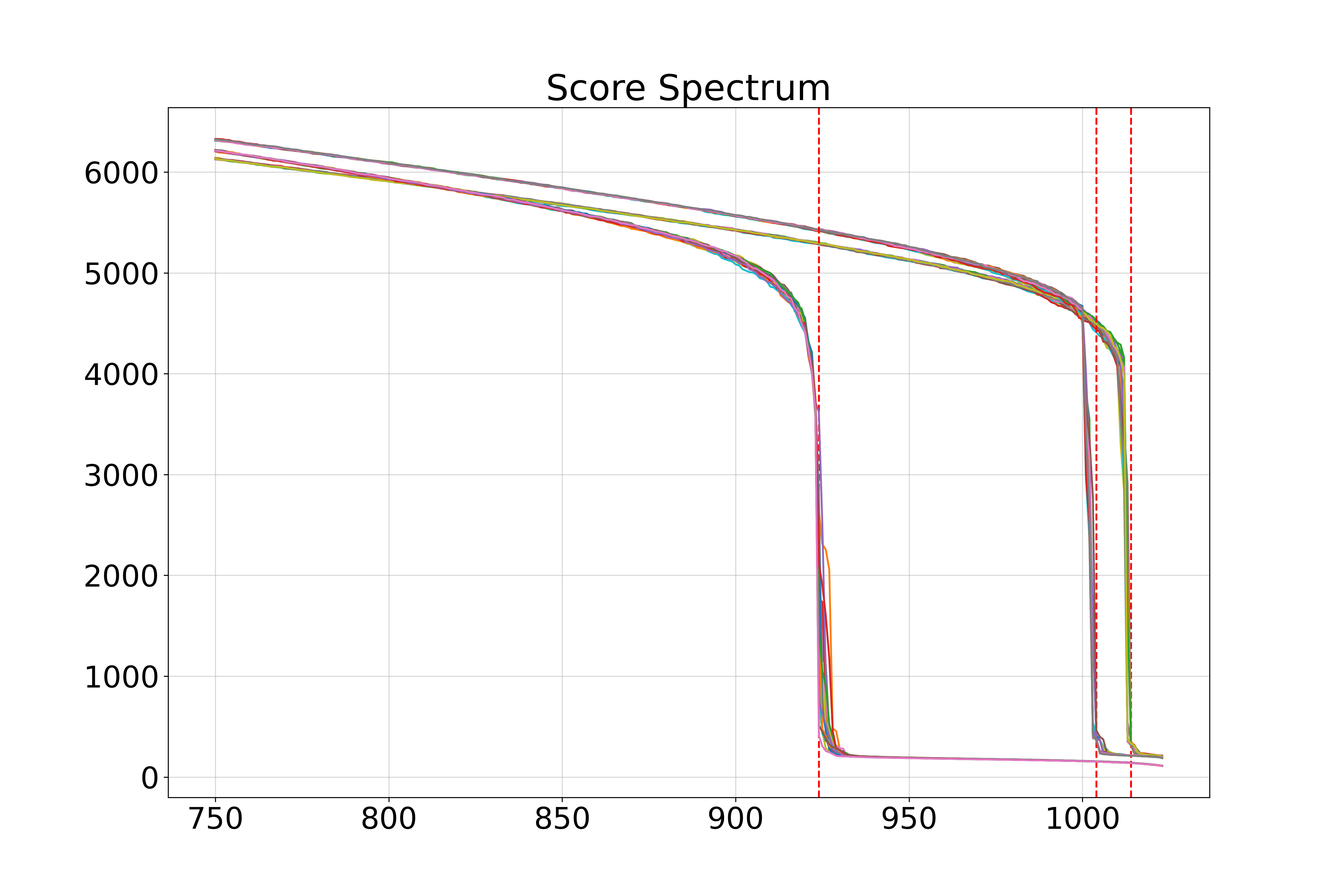
- Perform Singular Value Decomposition (SVD) on \( S \) to obtain singular values \( (s_i)_{i=1}^d \).
- Estimate \( \hat{k}(\mathbf{x}_0) = d - \arg\max_{i=1,\dots,d-1} (s_i - s_{i+1}) \).
- Estimated intrinsic dimension \( \hat{k}(\mathbf{x}_0) \).
Theoretical Results
Using the notion of tubular neighbourhood and Morse theory, we rigorously proved the following theorem, confirming our initial intuition. Full details of the proof are provided in Appendix D of the paper.
Theorem
Experiments
We validated our method on various datasets, both synthetic and real-world, comparing it with traditional intrinsic dimension estimation techniques.
Synthetic Manifolds
\( k \)-Spheres in 100 Dimensions
We generate \( k \)-dimensional spheres embedded in \( \mathbb{R}^{100} \) using random isometric embeddings.
- 10-Sphere (\( k = 10 \)): Estimated \( \hat{k} = 11 \)
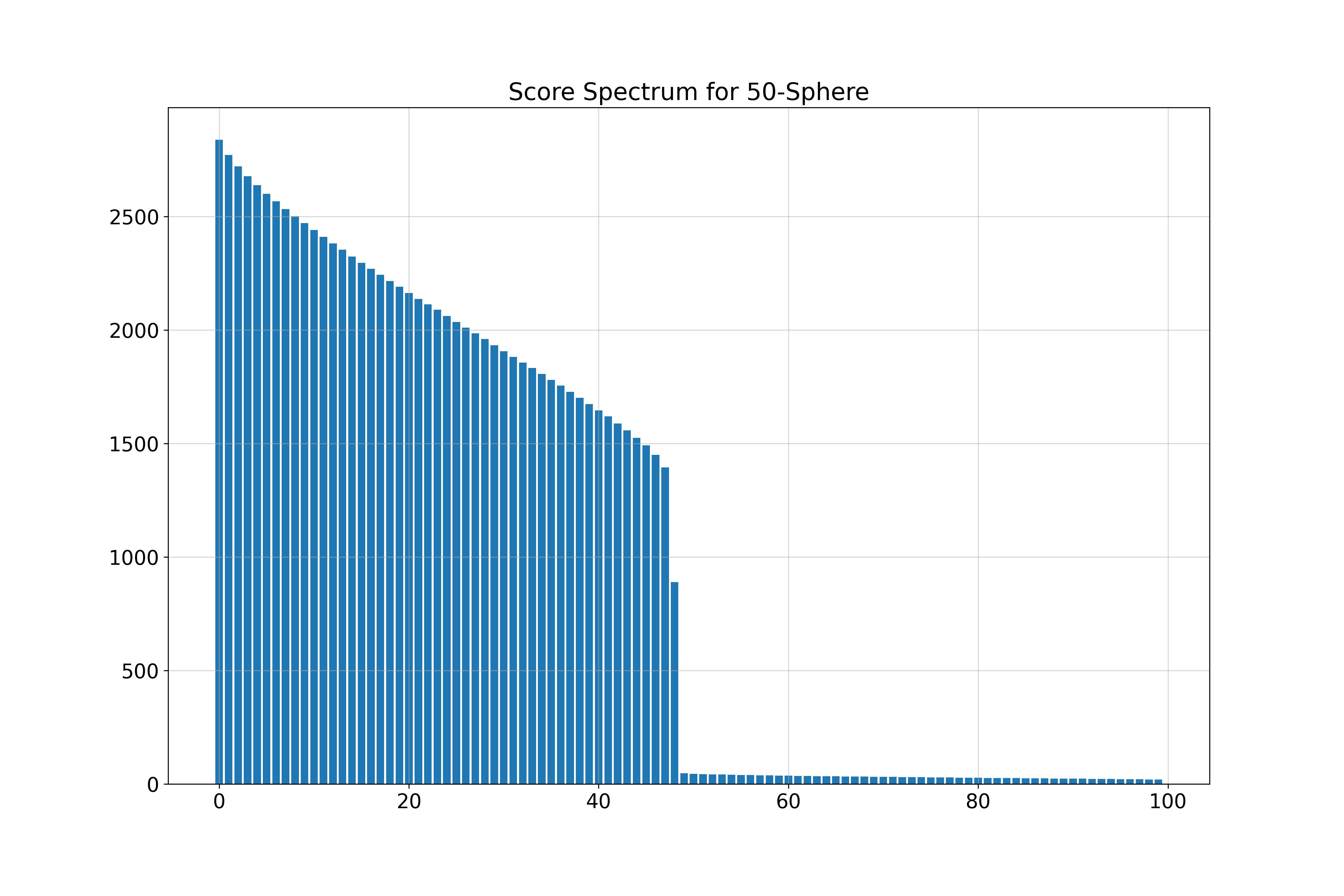
- 50-Sphere (\( k = 50 \)): Estimated \( \hat{k} = 51 \)
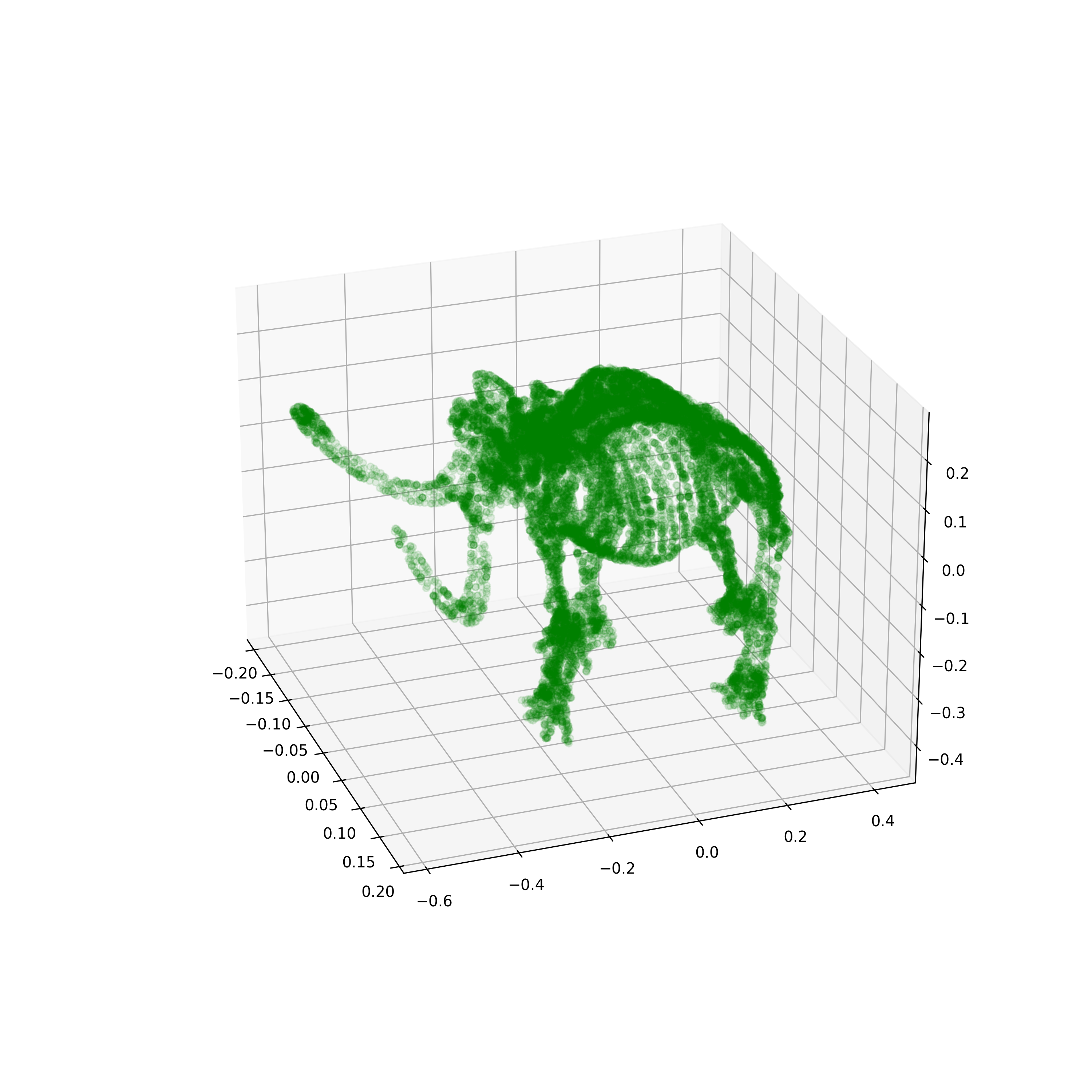
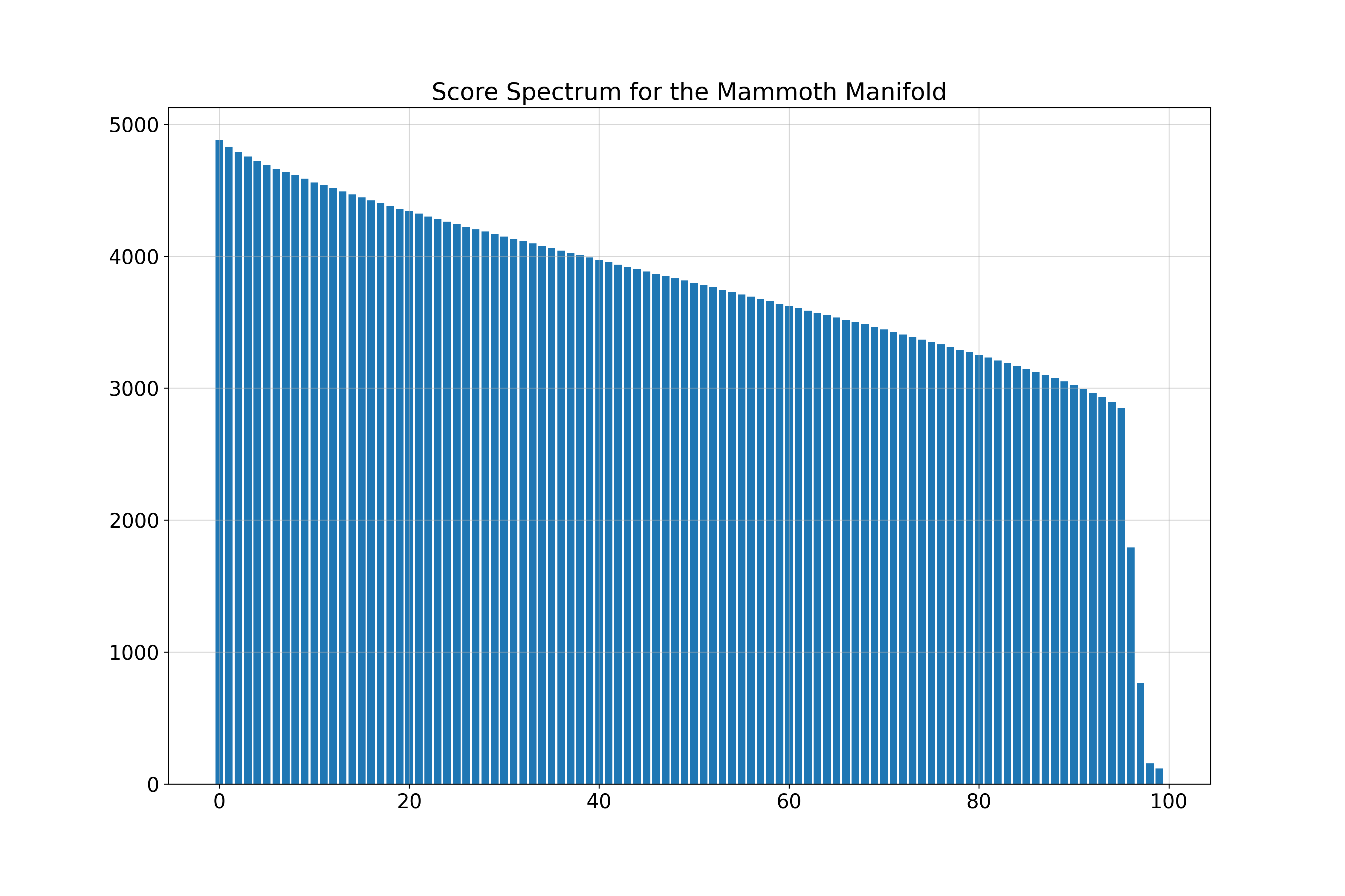
Mammoth Manifold
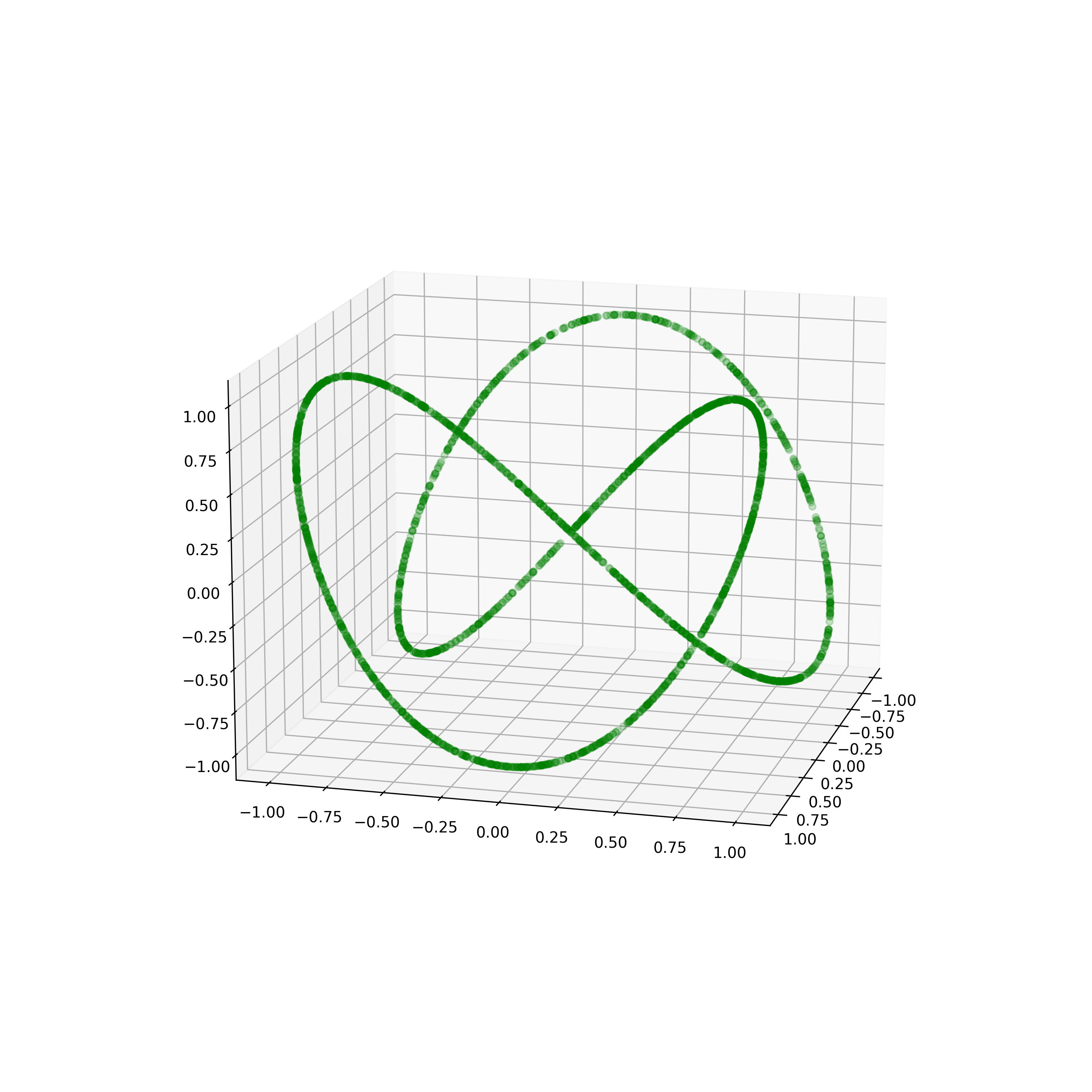
Spaghetti Line in 100 Dimensions
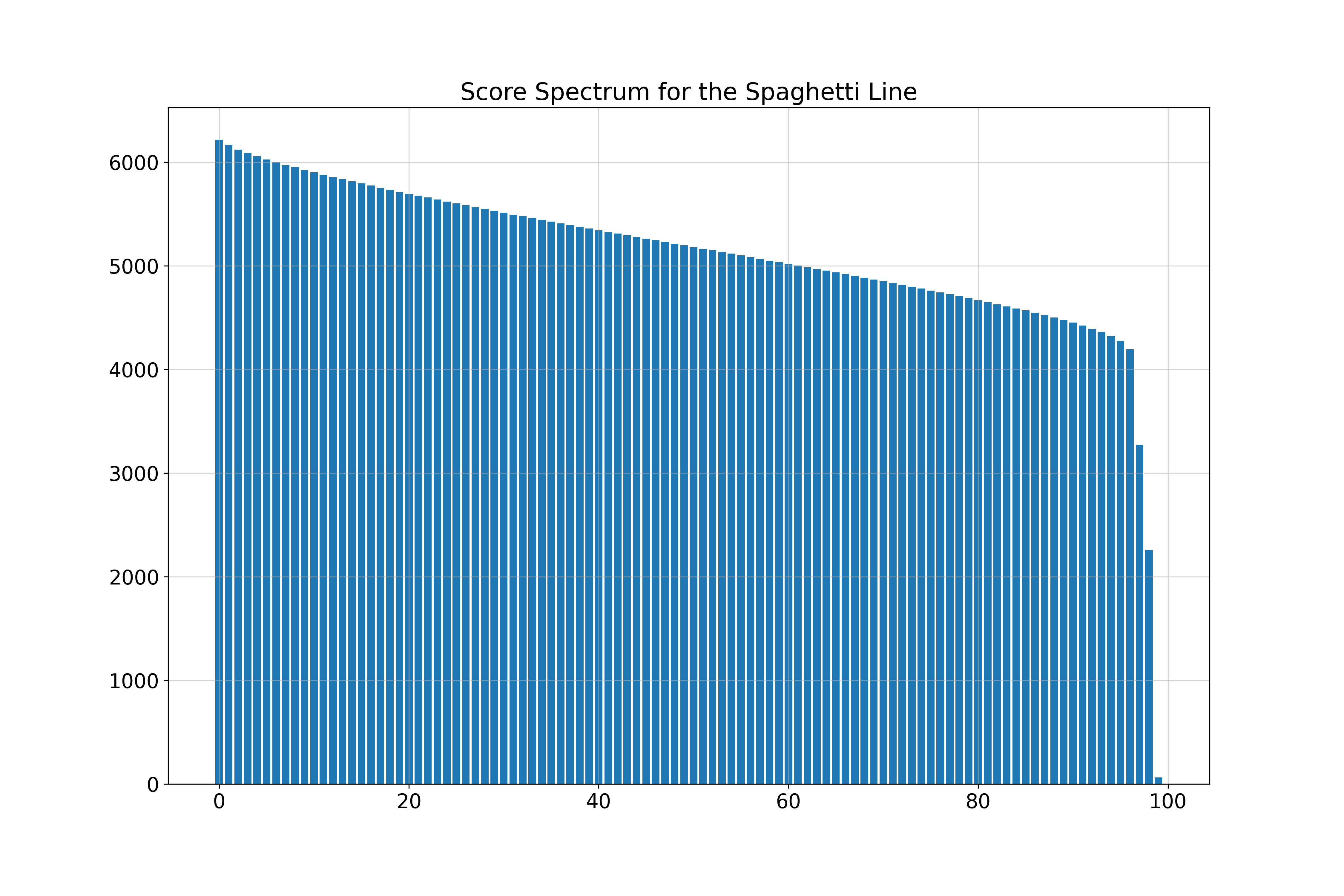
Union of Manifolds: 10-Sphere and 30-Sphere
We analyze a dataset composed of a union of two spheres.
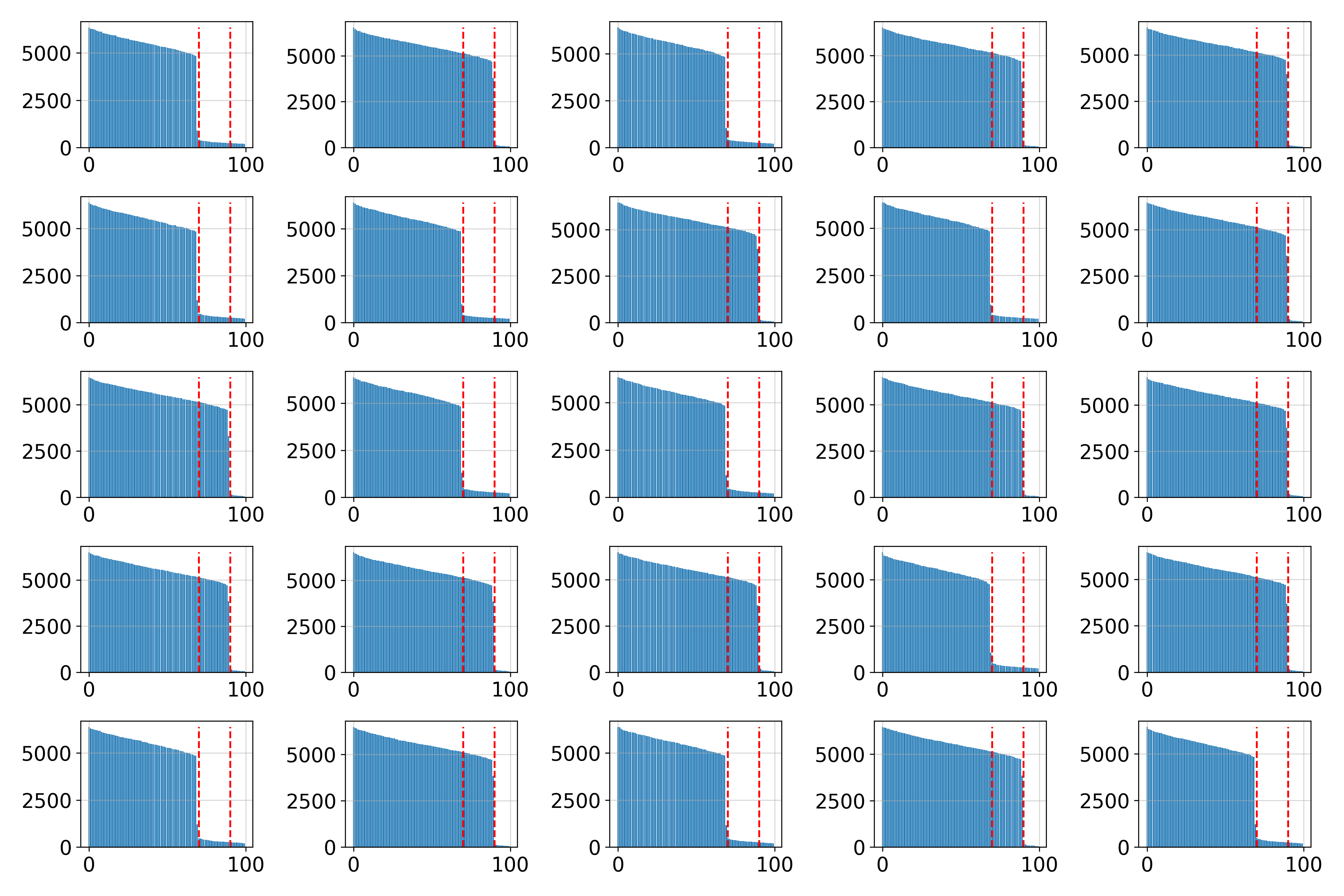
The estimated dimensions vary locally, reflecting the manifold’s structure.
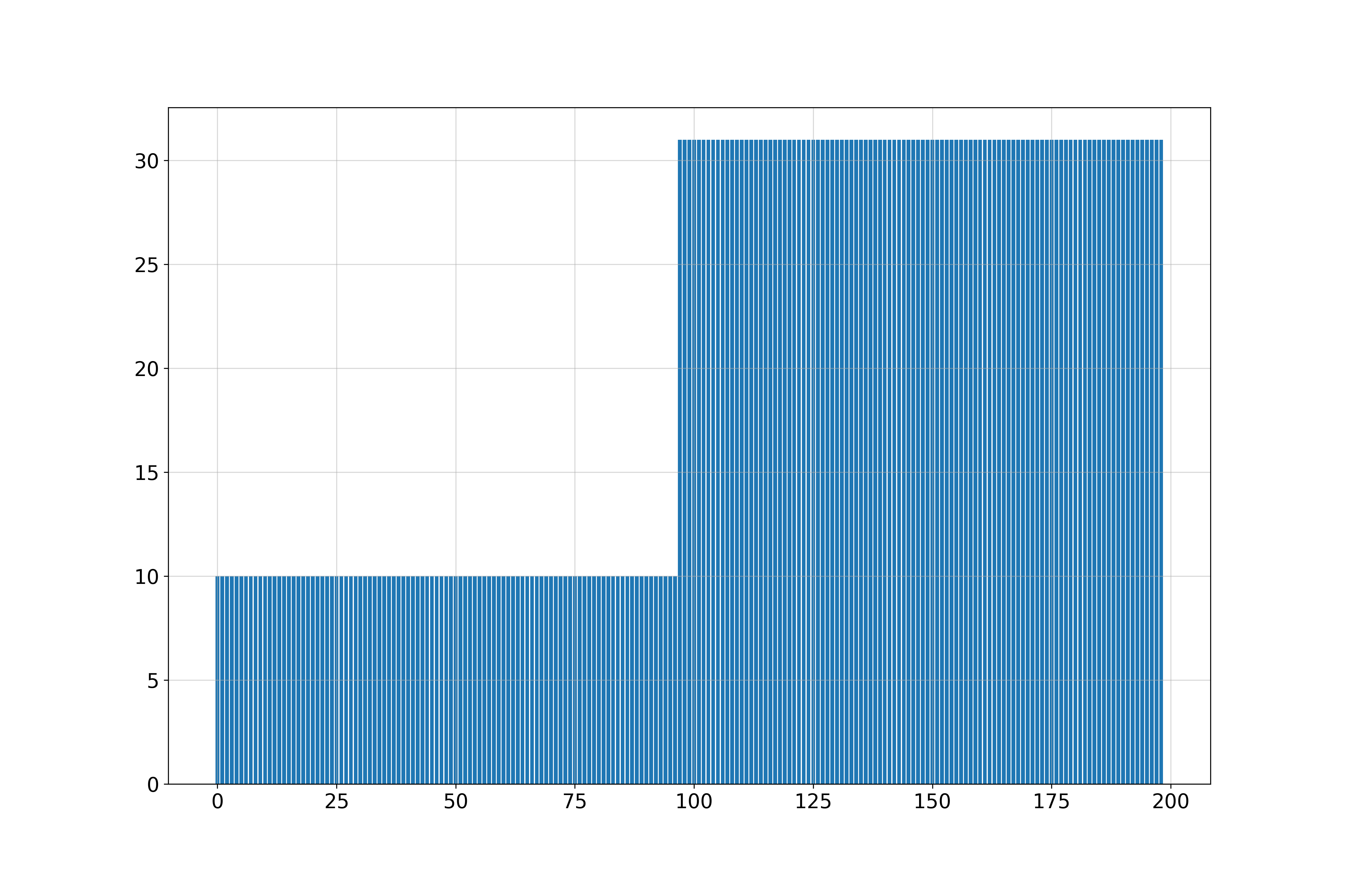
Image Manifolds
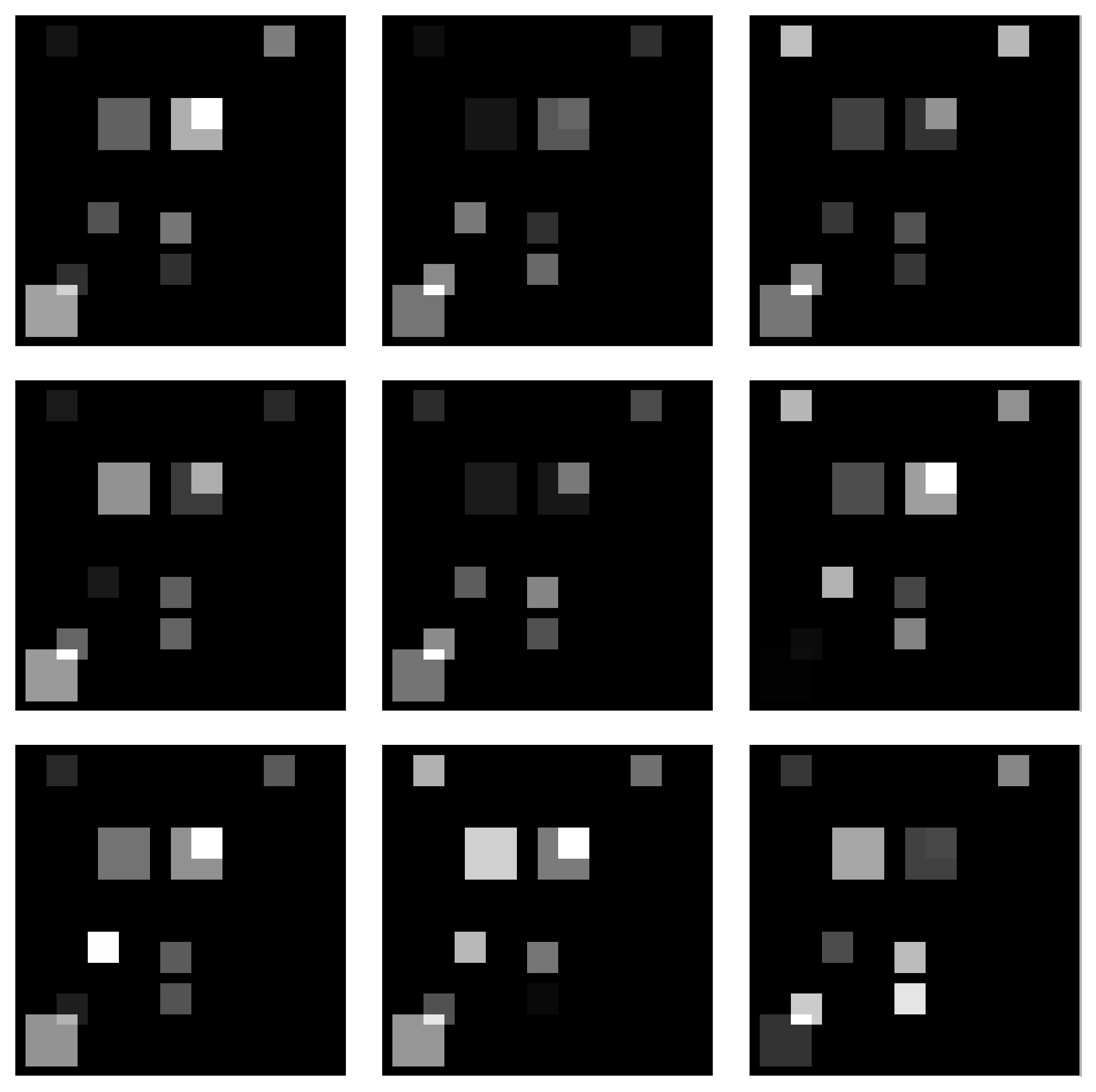
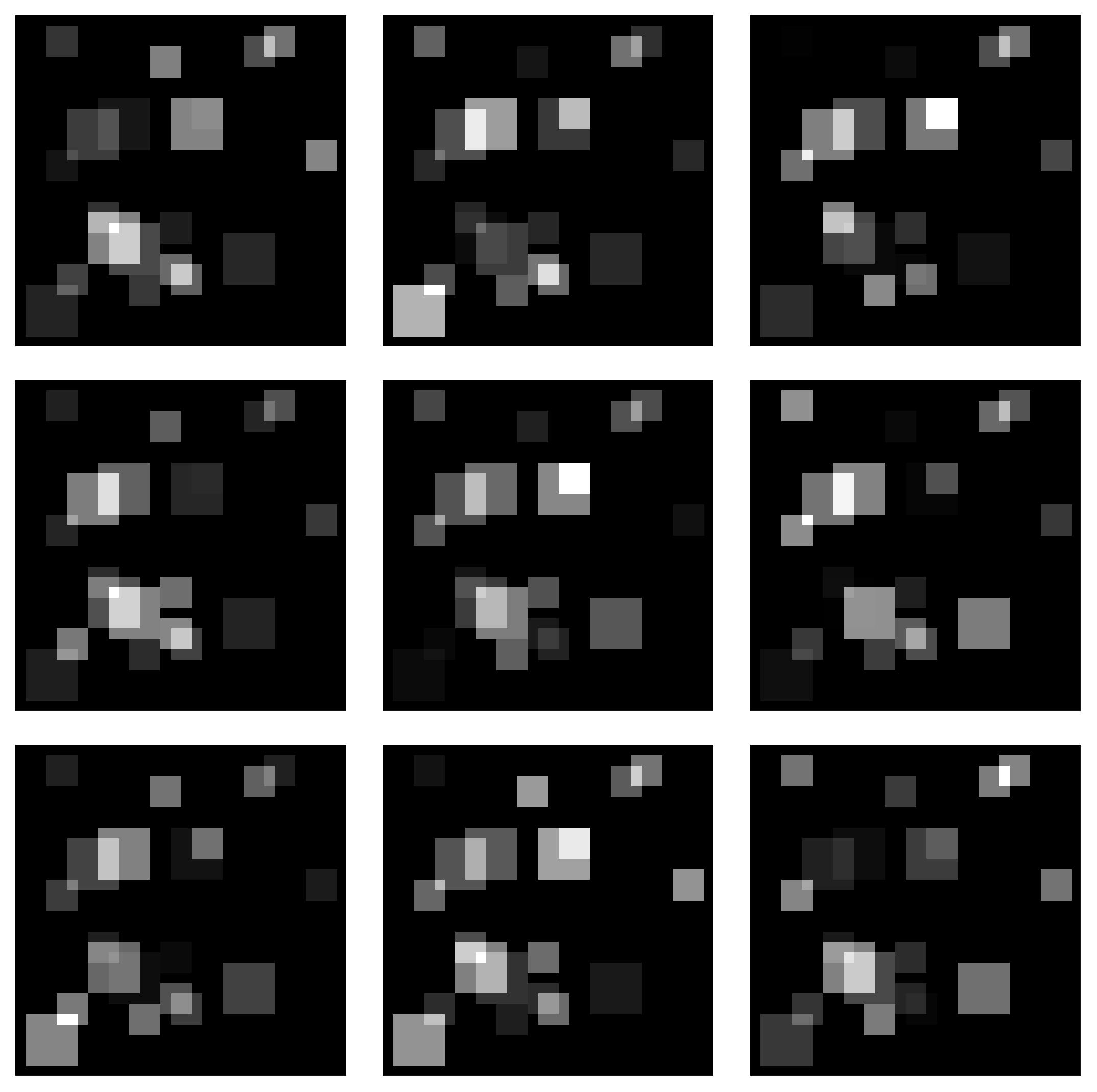
Square Manifold
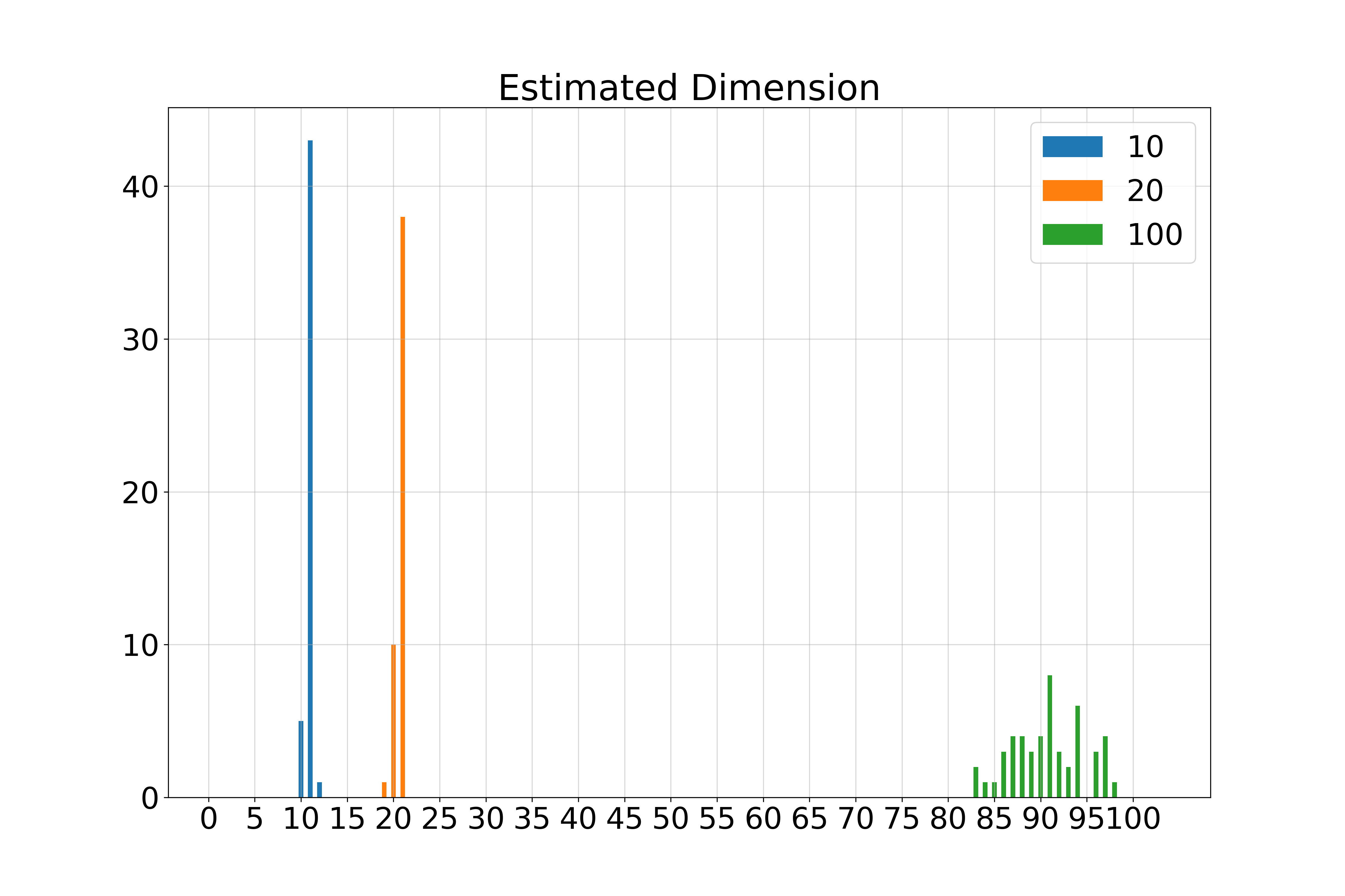
Samples from the Square Manifold for different dimensions:
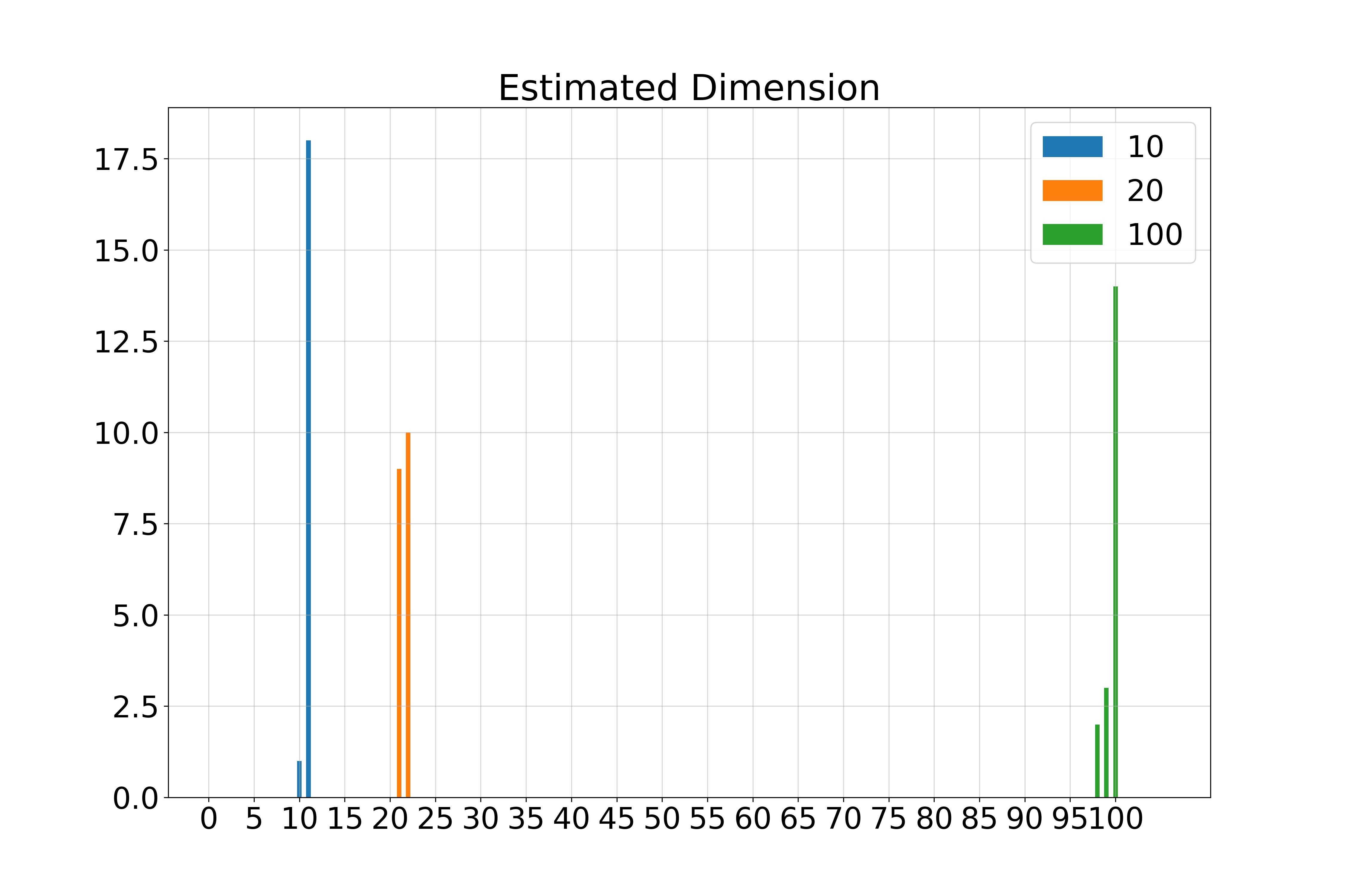
Spectra of singular values:
Gaussian Blobs Manifold
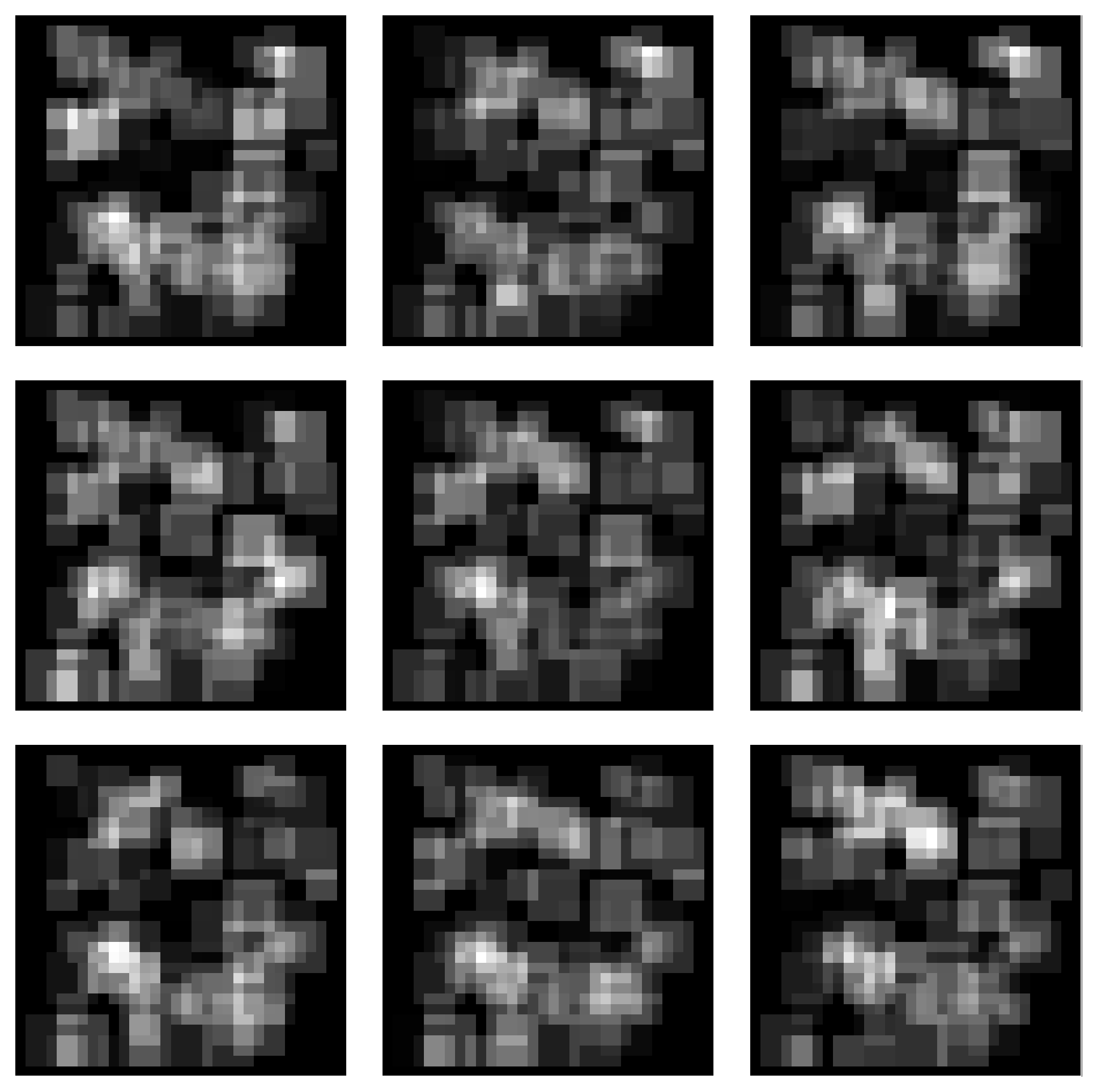
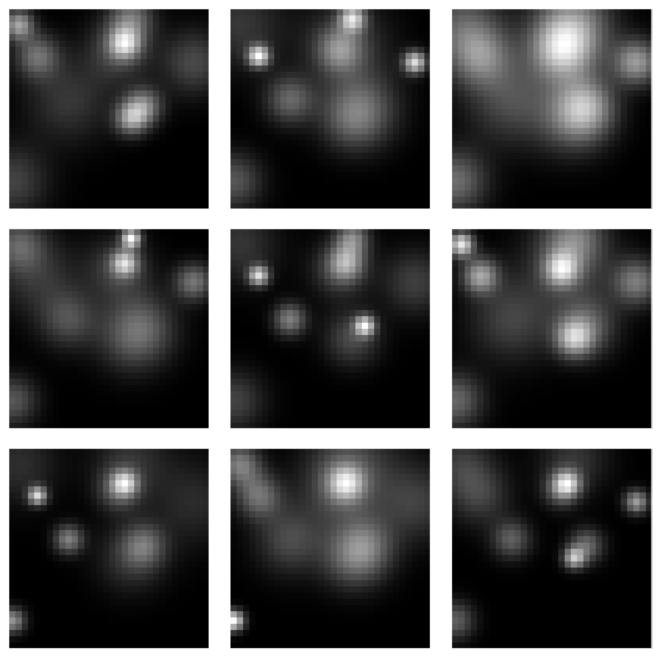
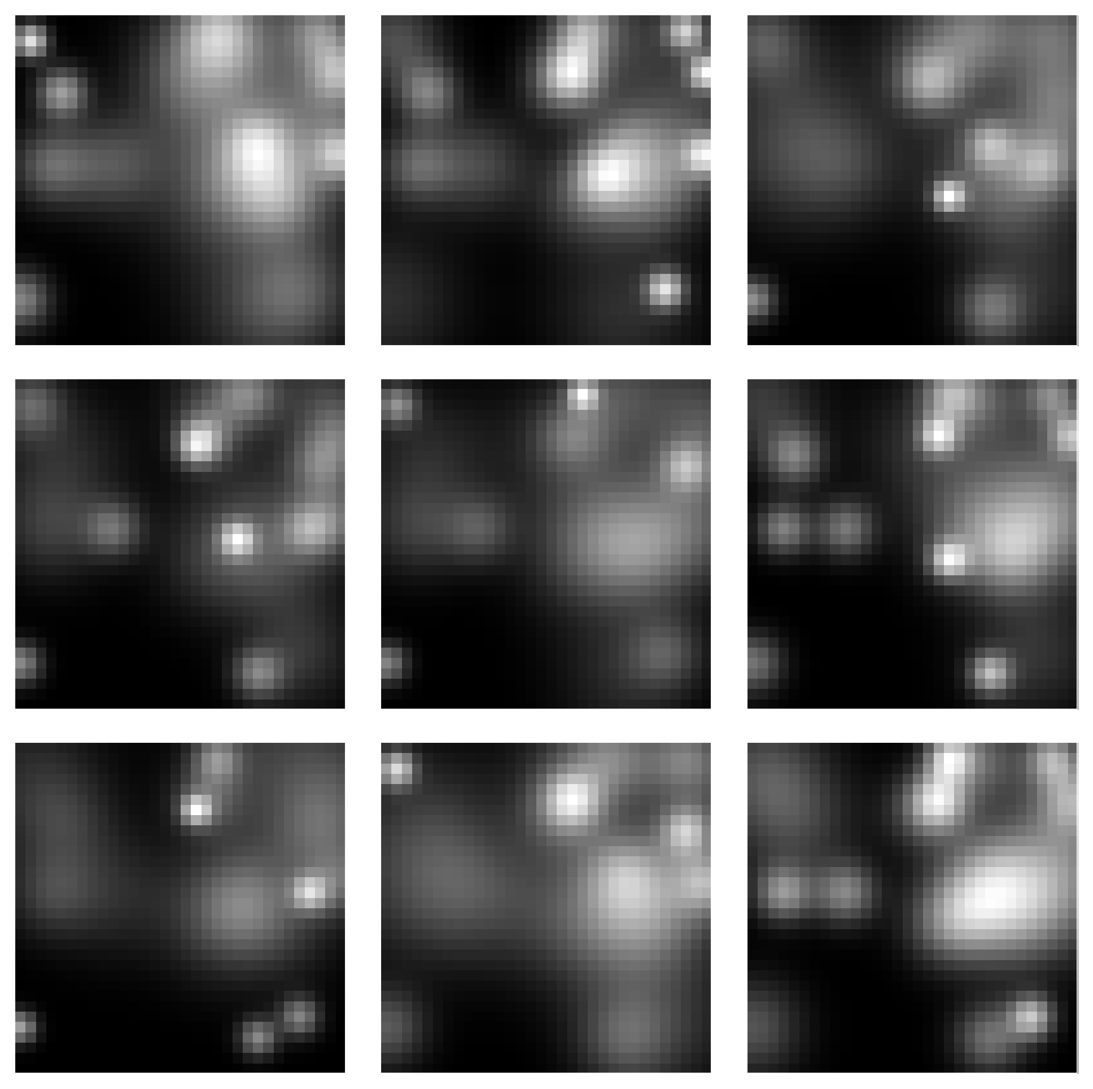
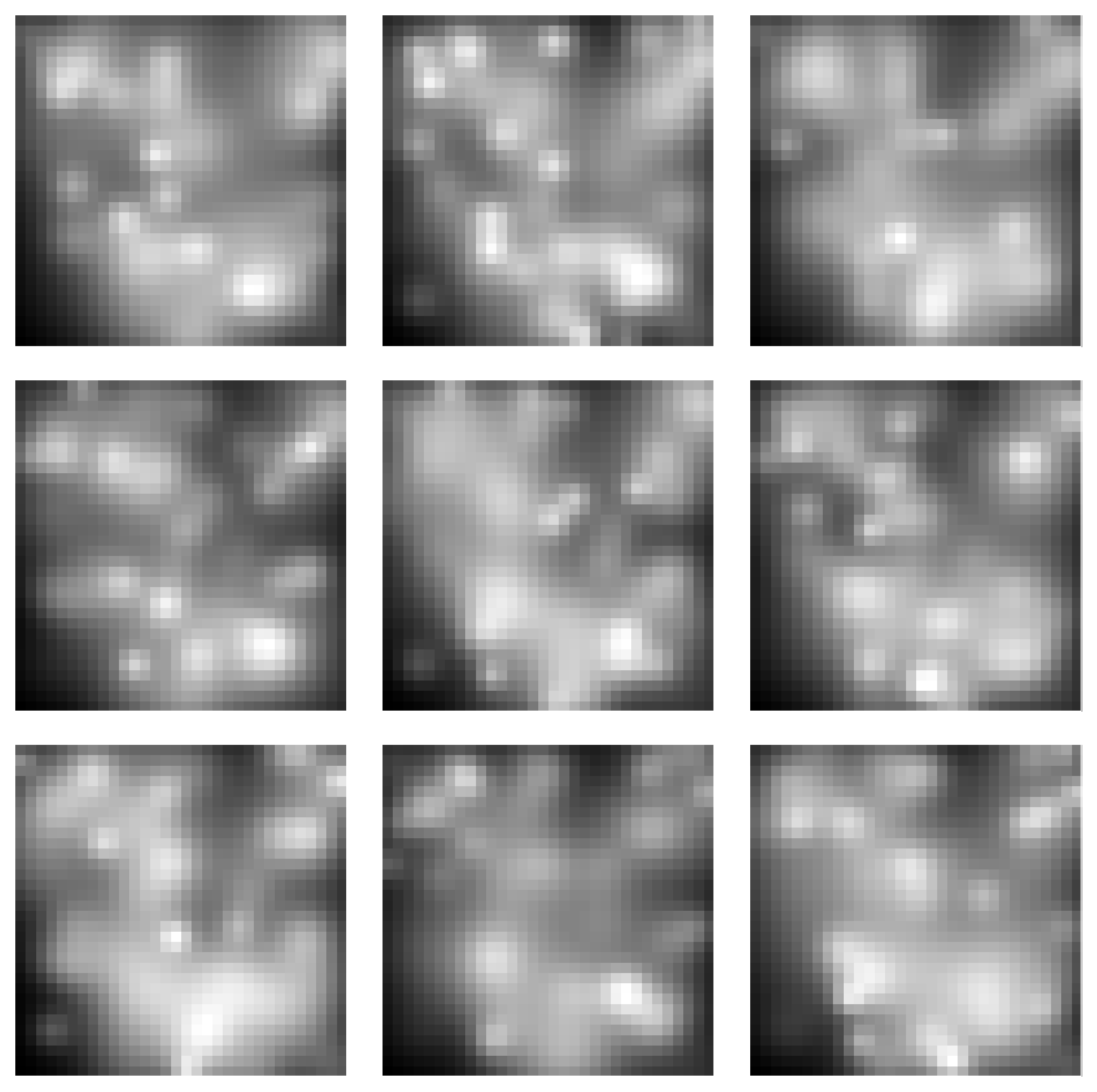
Samples from the Gaussian Blobs Manifold:
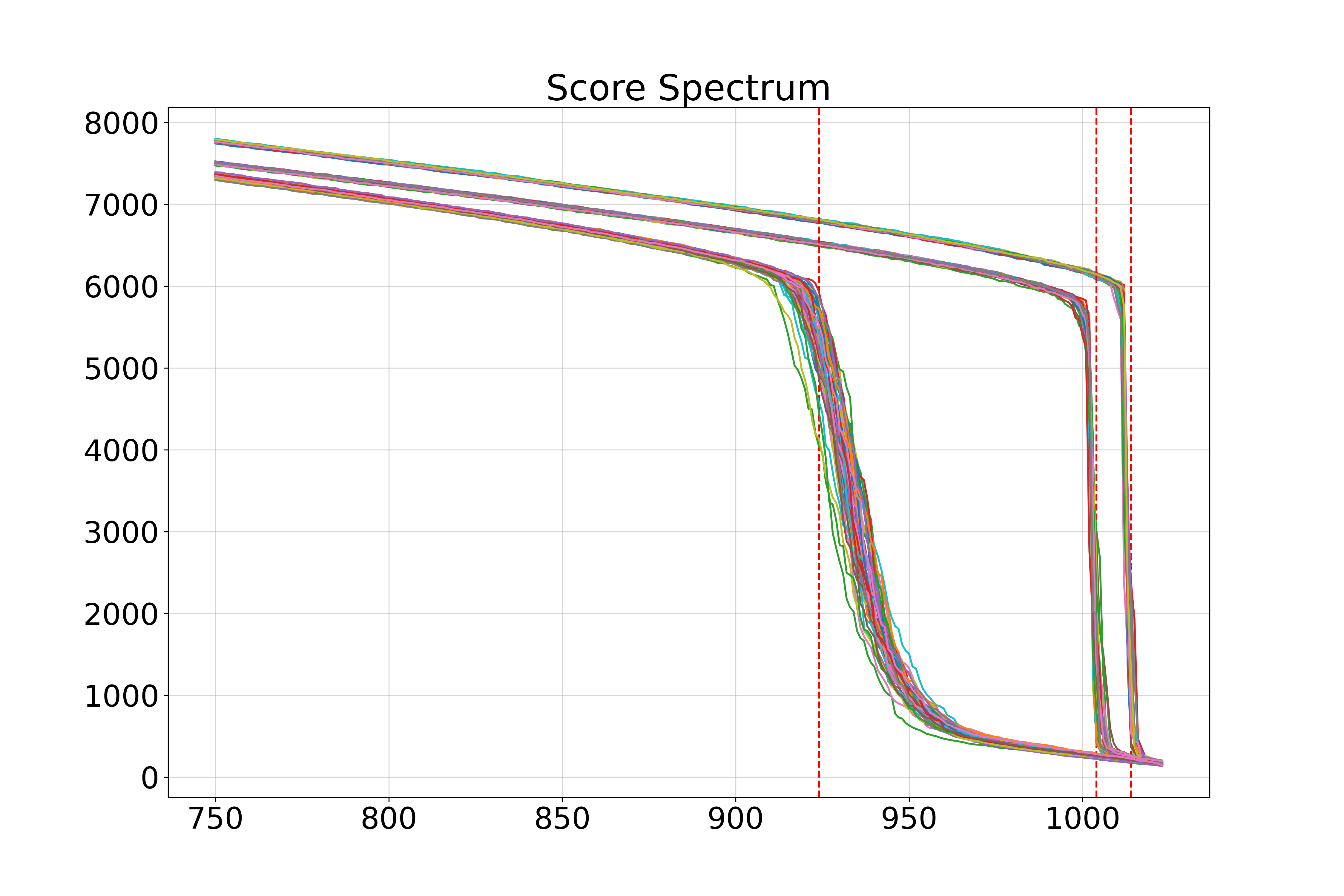
Spectra of singular values:
Real-World Data: MNIST
We applied our method to the MNIST handwritten digits dataset, analyzing each digit class separately.
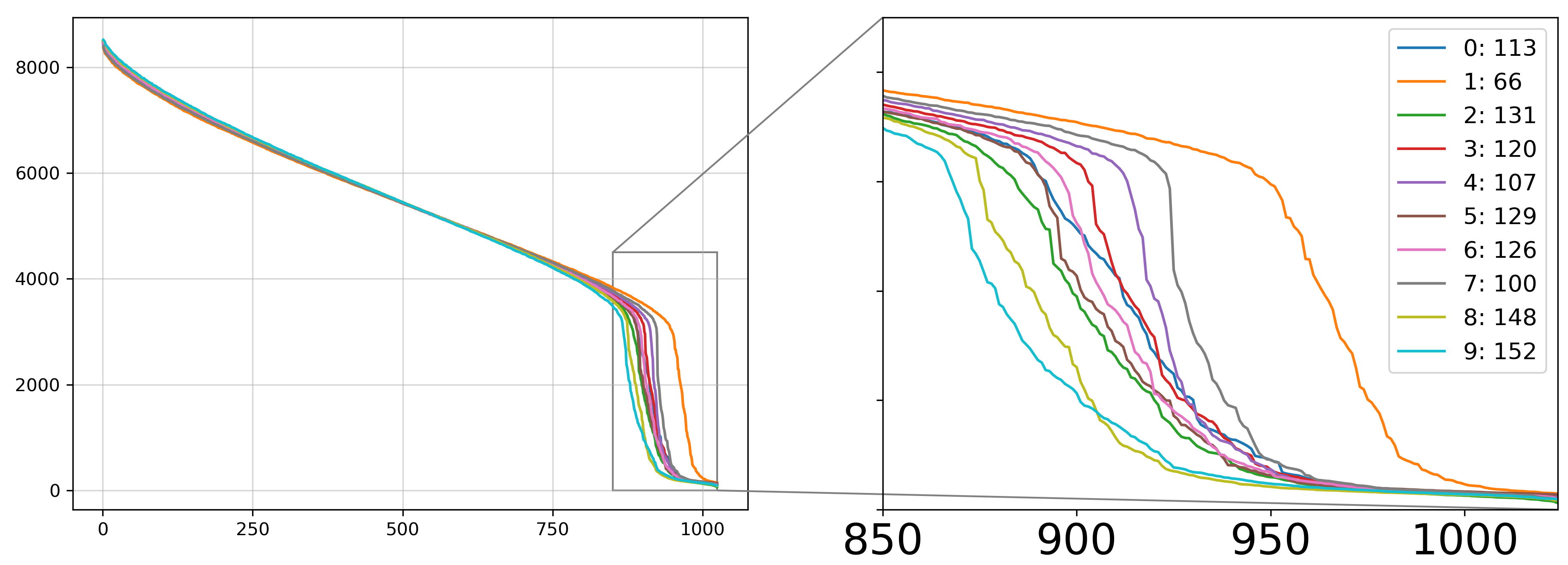
Figure: MNIST Score Spectra
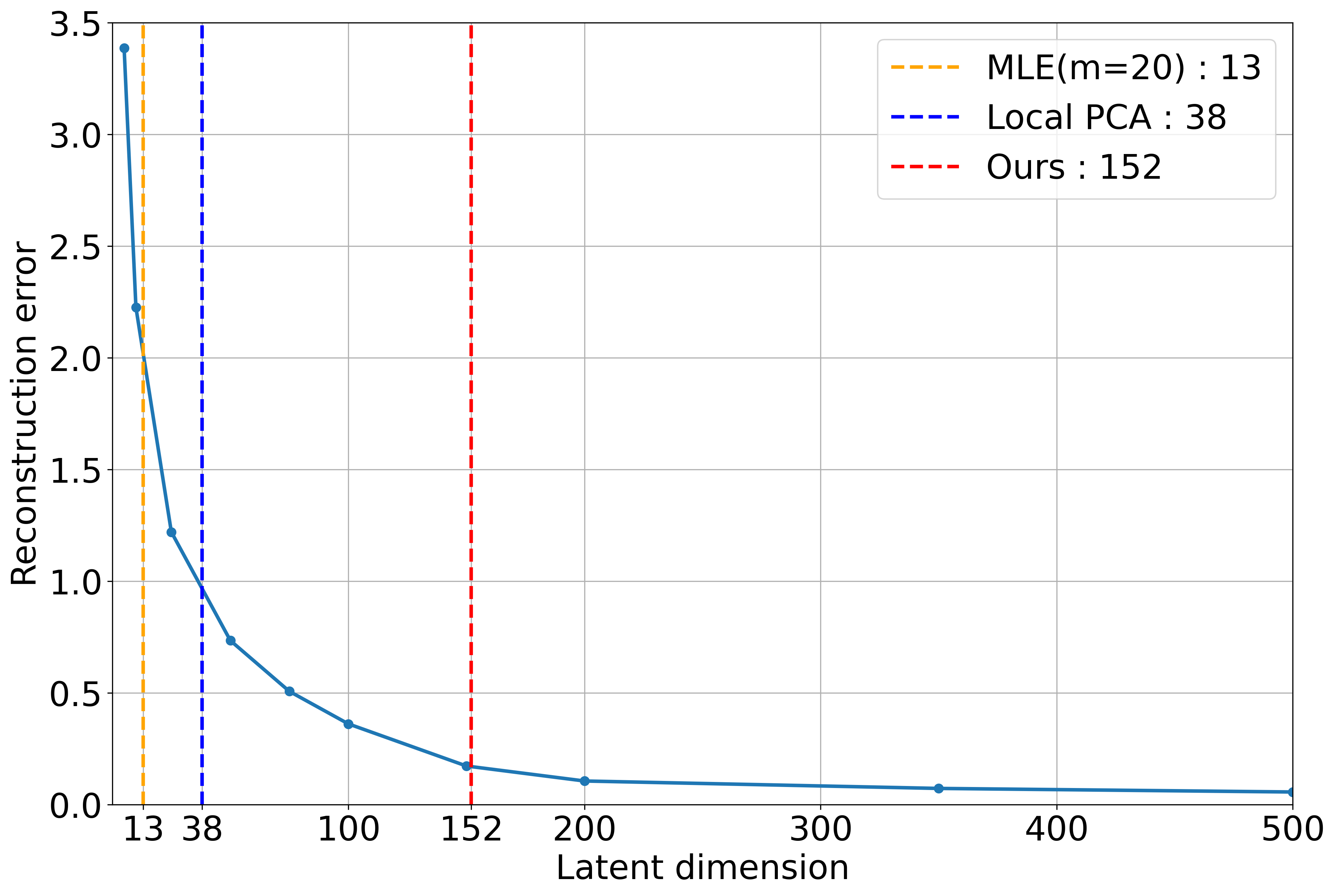
Figure: Autoencoder Validation
Estimated intrinsic dimensions for each digit:
| Digit | 0 | 1 | 2 | 3 | 4 | 5 | 6 | 7 | 8 | 9 |
|---|---|---|---|---|---|---|---|---|---|---|
| Estimated \( \hat{k} \) | 113 | 66 | 131 | 120 | 107 | 129 | 126 | 100 | 148 | 152 |
Summary of Experimental Results
We compared our method with other intrinsic dimension estimation techniques.
| Dataset | Ground Truth | Ours | MLE (m=5) | MLE (m=20) | Local PCA | PPCA |
|---|---|---|---|---|---|---|
| Euclidean Data Manifolds | ||||||
| 10-Sphere | 10 | 11 | 9.61 | 9.46 | 11 | 11 |
| 50-Sphere | 50 | 51 | 35.52 | 34.04 | 51 | 51 |
| Spaghetti Line | 1 | 1 | 1.01 | 1.00 | 32 | 98 |
| Image Manifolds | ||||||
| Squares (k=10) | 10 | 11 | 8.48 | 8.17 | 10 | 10 |
| Squares (k=20) | 20 | 22 | 14.96 | 14.36 | 20 | 20 |
| Squares (k=100) | 100 | 100 | 37.69 | 34.42 | 78 | 99 |
| Gaussian Blobs (k=10) | 10 | 12 | 8.88 | 8.67 | 10 | 136 |
| Gaussian Blobs (k=20) | 20 | 21 | 16.34 | 15.75 | 20 | 264 |
| Gaussian Blobs (k=100) | 100 | 98 | 39.66 | 35.31 | 18 | 985 |
| MNIST | ||||||
| All Digits | N/A | 152 | 14.12 | 13.27 | 38 | 706 |
Limitations
- Approximation Error: Caused by imperfect score approximation \( s_\theta(\mathbf{x}, t) \approx \nabla_{\mathbf{x}} \ln p_t(\mathbf{x}) \).
- Geometric Error: Arises when \( t \) isn't sufficiently small, leading to:
- Increased tangential components of the score vector.
- Differences in normal spaces across sampled points due to manifold curvature.
Conclusions
- Our estimator offers accurate intrinsic dimension estimates even for high-dimensional manifolds, indicating superior statistical efficiency compared to traditional methods.
- This improvement is credited to the inductive biases of the neural network estimating the score function, the critical quantity for intrinsic dimension estimation.
- Our theoretical results show that the diffusion model approximates the normal bundle of the manifold, providing more information than just the intrinsic dimension.
- We can potentially use a trained diffusion model to extract other important properties of the data manifold, such as curvature.