Score-based Pullback Riemannian Geometry
Overview
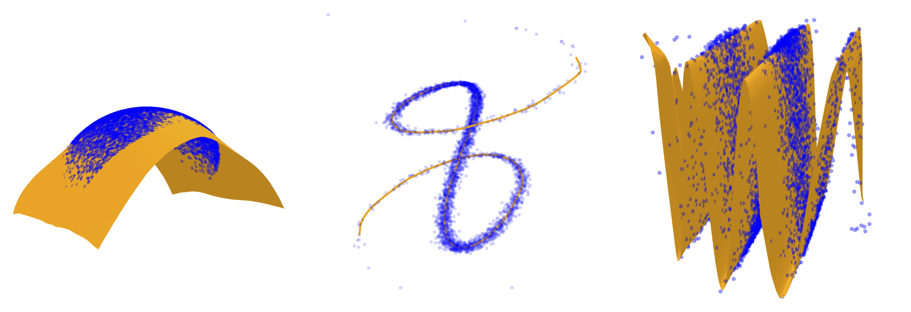
In our work, we propose a score-based pullback Riemannian metric, giving closed-form geodesics and interpretable autoencoding, capturing the intrinsic dimensionality & geometry of data!
We show that this geometry can naturally be extracted by adapting the normalizing flow framework with isometry regularization and base distribution anisotropy.
Model Definition and Training
We introduce two key modifications to the Normalizing Flow framework that allow us to construct Riemannian geometry from unimodal densities \(p: \mathbb{R}^d \rightarrow \mathbb{R}^d \) of the form \[p(\mathbf{x}) \propto e^{-\psi(\varphi(\mathbf{x}))} \] where \(\psi: \mathbb{R}^d \rightarrow \mathbb{R}^d\) is a smooth strongly convex function and \(\phi: \mathbb{R}^d \rightarrow \mathbb{R}^d\) is a diffeomorphism.
- Anisotropic Base Distribution: Instead of using a fixed isotropic Gaussian as the base distribution, we parameterize the diagonal elements of the covariance matrix \(\mathbf{\Sigma}_{\theta_1}\) of the base distribution. This allows the model to learn an anisotropic Gaussian, capturing variations along different directions of the data manifold.
- Isometry Regularization: We encourage the flow \(\phi_{\theta_2}\) to be approximately isometric with respect to the Euclidean metric. This is achieved by adding a regularization term to the training objective, promoting the preservation of distances and angles during the transformation. This leads to more stable and interpretable manifold mappings.
Normalizing Flow Density and Training Objective
- \( \phi_{\theta_2}: \mathbb{R}^d \rightarrow \mathbb{R}^d \) is an invertible transformation (diffeomorphism) parameterized by \( \theta_2 \).
- \( D_{\mathbf{x}} \phi_{\theta_2} \) is the Jacobian matrix of \( \phi_{\theta_2} \) at point \( \mathbf{x} \).
- \( p_{\mathcal{Z}}(\mathbf{z}) \) is the base density evaluated at \( \mathbf{z} = \phi_{\theta_2}(\mathbf{x}) \).
Base Density
The base density \( p_{\mathcal{Z}}(\mathbf{z}) \) is chosen as the density of an anisotropic Gaussian distribution with a learnable covariance matrix \( \mathbf{\Sigma}_{\theta_1} \): \[ p_{\mathcal{Z}}(\mathbf{z}) = \frac{1}{(2\pi)^{d/2} \det(\mathbf{\Sigma}_{\theta_1})^{1/2}} \exp\left( -\frac{1}{2} \mathbf{z}^\top \mathbf{\Sigma}_{\theta_1}^{-1} \mathbf{z} \right). \]Training Objective
Our training objective combines the negative log-likelihood of the data under the model with an isometry regularization term: \[ \mathcal{L}(\theta_1, \theta_2) = \mathbb{E}_{\mathbf{x} \sim p_{\text{data}}} \left[ -\log p_{\theta_1, \theta_2}(\mathbf{x}) \right] + \lambda_{\text{iso}} \, \mathbb{E}_{\mathbf{x} \sim p_{\text{data}}} \left[ \left\| (D_{\mathbf{x}} \phi_{\theta_2})^\top D_{\mathbf{x}} \phi_{\theta_2} - \mathbf{I}_d \right\|_F^2 \right], \] where:- Negative Log-Likelihood Term: Encourages the model to fit the data distribution by minimizing the negative log-likelihood. Expanding this term, we get: \[ \begin{align*} \mathbb{E}_{\mathbf{x} \sim p_{\text{data}}} \left[ - \log p_{\theta_1, \theta_2}(\mathbf{x}) \right] &= \mathbb{E}_{\mathbf{x} \sim p_{\text{data}}} \left[ - \log p_{\mathcal{Z}} \left( \phi_{\theta_2}(\mathbf{x}) \right) - \log \left| \det \left( D_{\mathbf{x}} \phi_{\theta_2} \right) \right| \right] \\ &= \mathbb{E}_{\mathbf{x} \sim p_{\text{data}}} \left[ \frac{d}{2} \log (2\pi) + \frac{1}{2} \log \det \left( \mathbf{\Sigma}_{\theta_1} \right) + \frac{1}{2} \phi_{\theta_2}(\mathbf{x})^\top \mathbf{\Sigma}_{\theta_1}^{-1} \phi_{\theta_2}(\mathbf{x}) - \log \left| \det \left( D_{\mathbf{x}} \phi_{\theta_2} \right) \right| \right]. \end{align*} \]
- Isometry Regularization Term: Penalizes deviations from isometry, encouraging the transformation \( \phi_{\theta_2} \) to be approximately length-preserving. Here \( \lambda_{\text{iso}} > 0 \) is the regularization weight, \( \|\cdot\|_F \) denotes the Frobenius norm, \( ( D_{\mathbf{x}} \phi_{\theta_2} )^\top D_{\mathbf{x}} \phi_{\theta_2} \) is the Gram matrix of the Jacobian and \( \mathbf{I}_d \) is the \( d \times d \) identity matrix.
Connection to Riemannian Geometry
- A learned diffeomorphism \( \phi_{\theta_2}: \mathbb{R}^d \rightarrow \mathbb{R}^d \), representing the transformation learned by the flow.
- A learned strongly convex function \( \psi: \mathbb{R}^d \rightarrow \mathbb{R} \), associated with the anisotropic Gaussian base distribution.
Constructing the pullback Riemannian Metric:
We define a pullback metric: on the data space \( \mathbb{R}^d \) using the composition of the gradient of \( \psi \) with the learned diffeomorphism \( \phi_{\theta_2} \): \[ g_{\mathbf{x}}( \mathbf{v}, \mathbf{w} ) = \left( D_{\mathbf{x}} \nabla \psi \circ \phi_{\theta_2}[ \mathbf{v} ],\ D_{\mathbf{x}} \nabla \psi \circ \phi_{\theta_2}[ \mathbf{w} ] \right)_2, \] where:- \( D_{\mathbf{x}} \nabla \psi \circ \phi_{\theta_2} \) is the Jacobian of \( \nabla \psi \circ \phi_{\theta_2} \) at \( \mathbf{x} \).
- \( \mathbf{v}, \mathbf{w} \in T_{\mathbf{x}} \mathbb{R}^d \) are tangent vectors at \( \mathbf{x} \).
- \( (\cdot, \cdot )_2 \) denotes the standard Euclidean inner product.
The defined pullback metric is related to pullback metric of the score function of the distribution. It enables the computation of geodesics and other manifold mappings that pass through regions of high data density in closed form.
Moreover, the learned covariance matrix \( \mathbf{\Sigma}_{\theta_1} \) from \( \psi \) enables the construction of a Riemannian Auto-encoder (RAE). The latent dimensions associated with significant variance (i.e., large \( \sigma_i^2 \)) are used for the construction of a Riemannian Auto-encoder that captures both the geometry and the dimensionality of the data manifold.
For more details on the connection of our defined metric to the pullback metric of the score function and the construction of the Riemannian Auto-encoder, please refer to sections 3-5 of the paper.
Experimental Results
Riemannian Auto-encoder
1D and 2D Manifolds
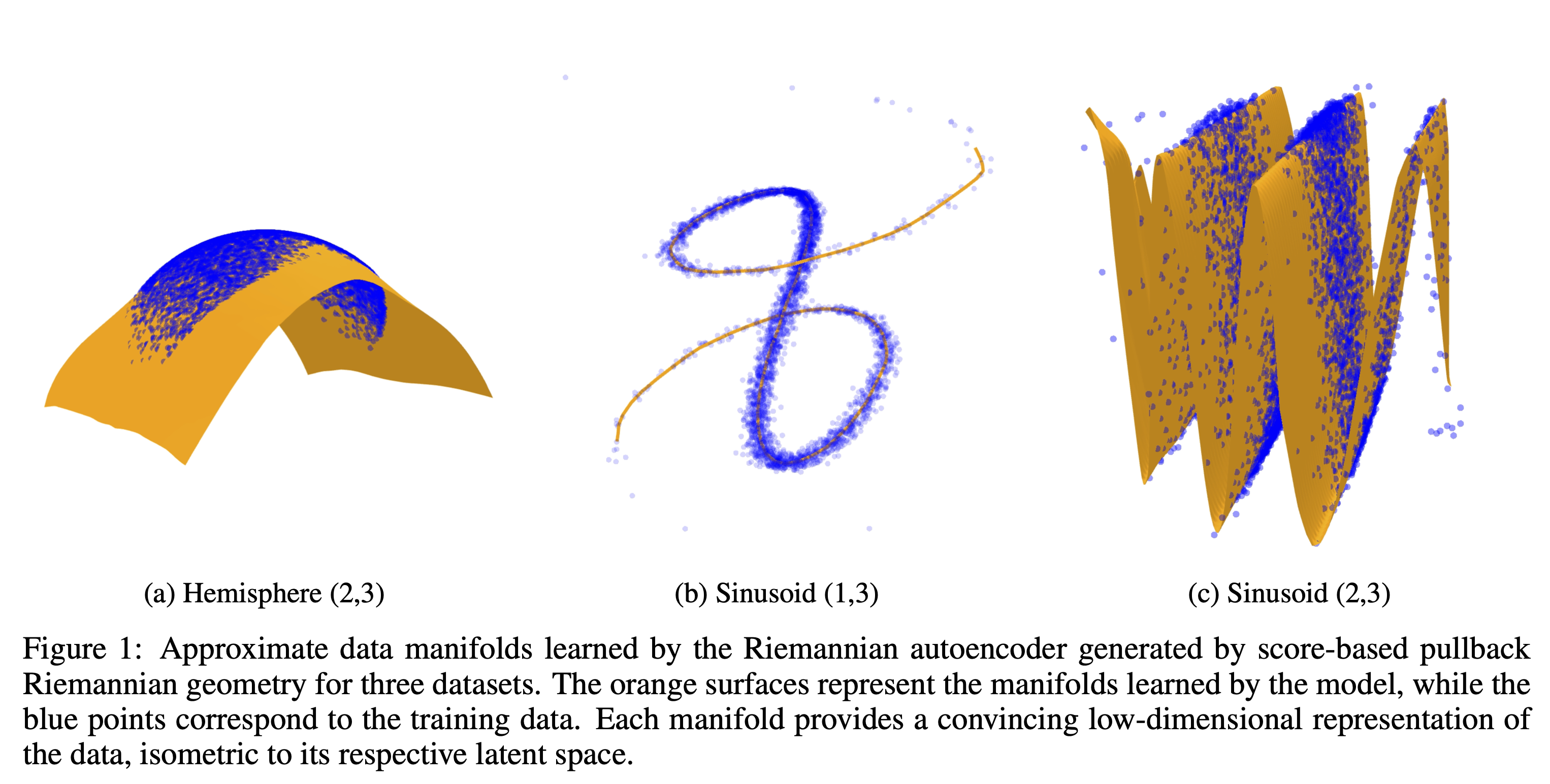
The Riemannian Autoencoder effectively learns low-dimensional representations, as shown in the approximations below.
Sinusoid(1, 100) Data Manifold Approximation
Our method effectively captures low dimensional manifolds embeeded in high dimensional spaces, such as the Sinusoid(1, 100) dataset, as seen in the following figure.
Higher-Dimensional Manifolds (5D Embedded in 20D)
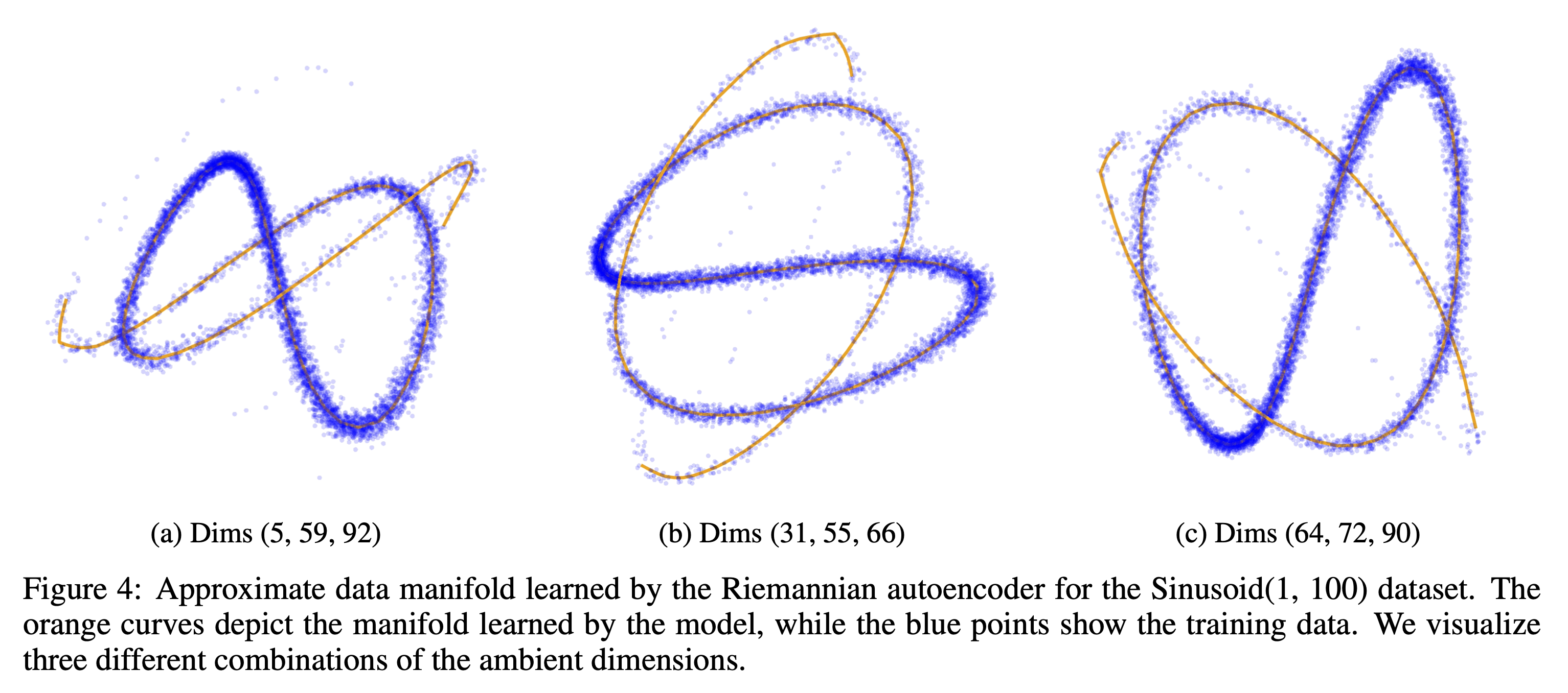
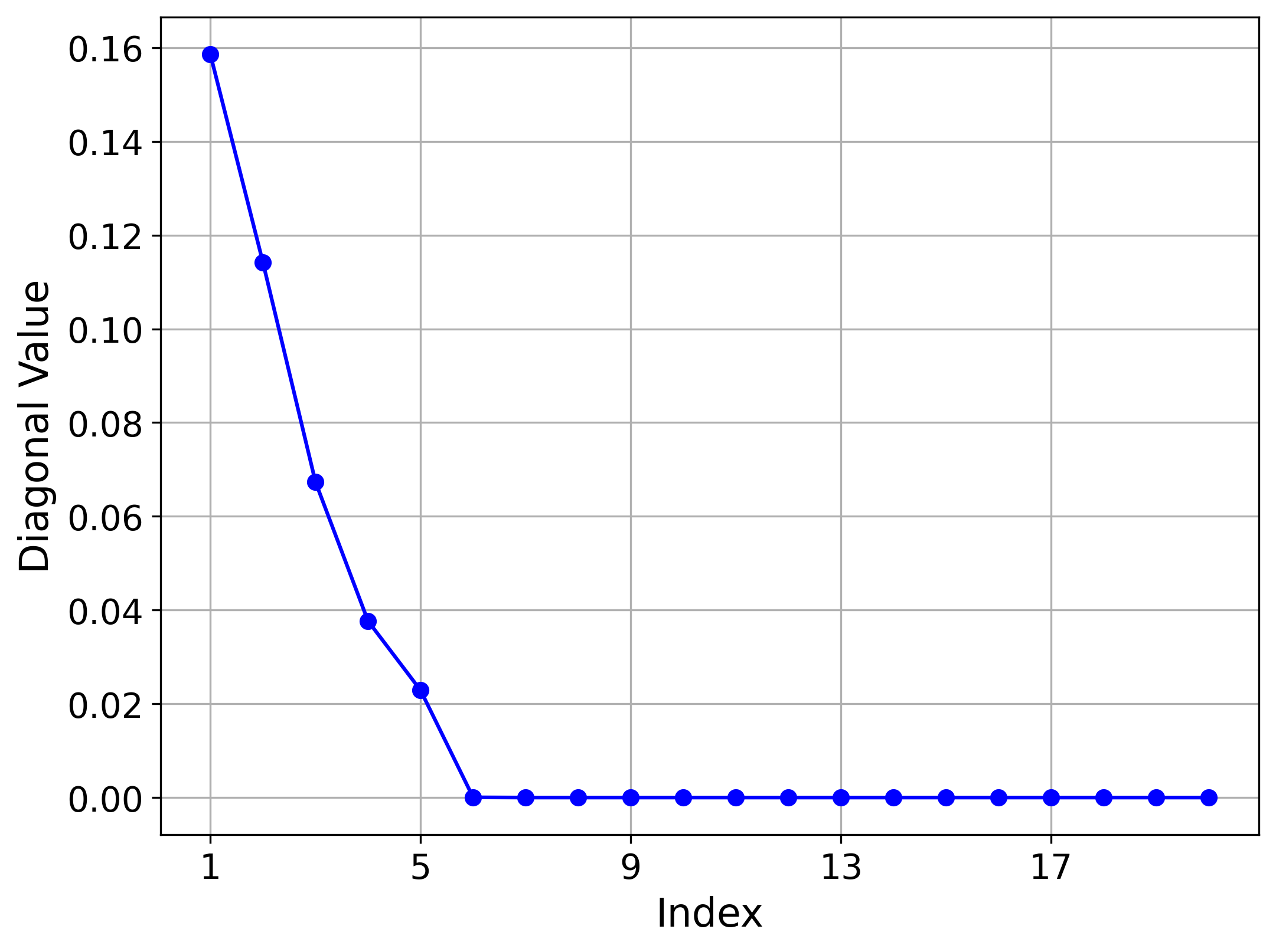
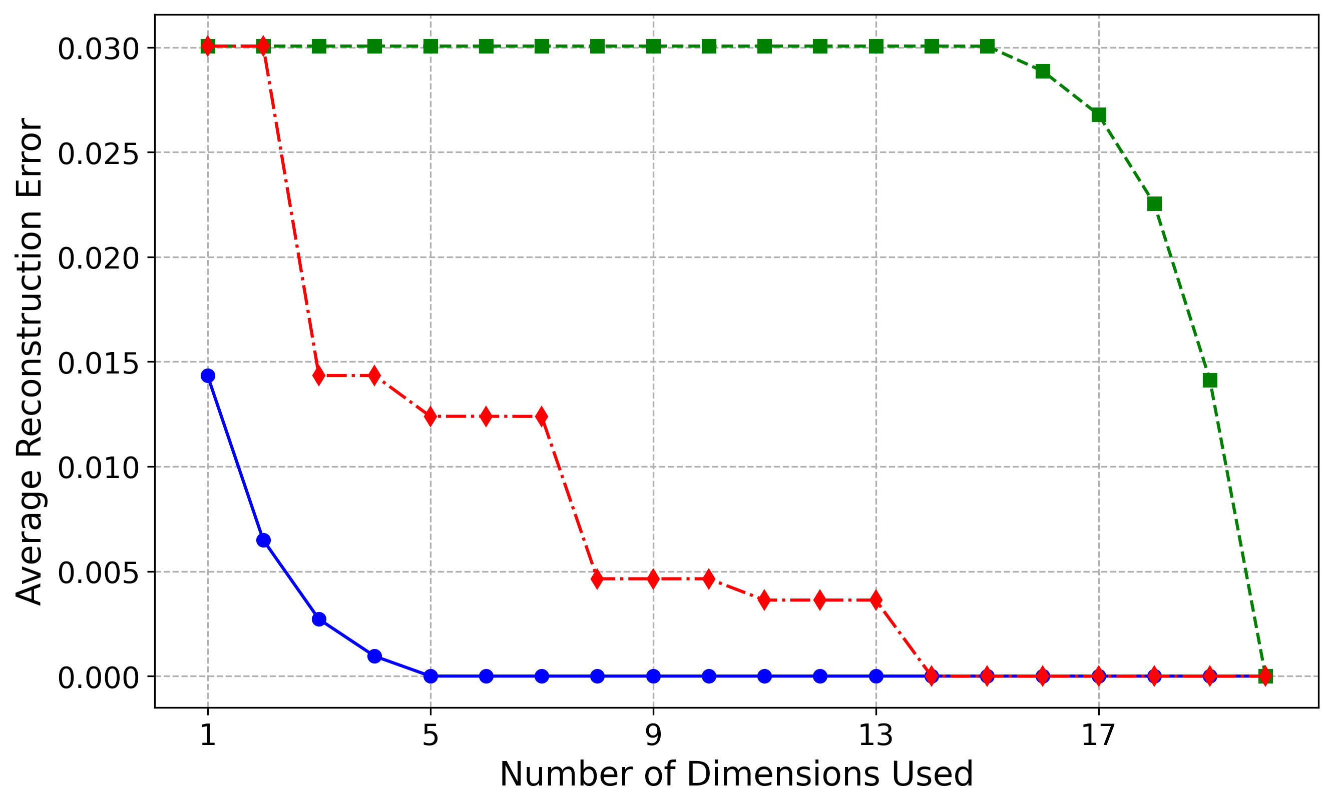
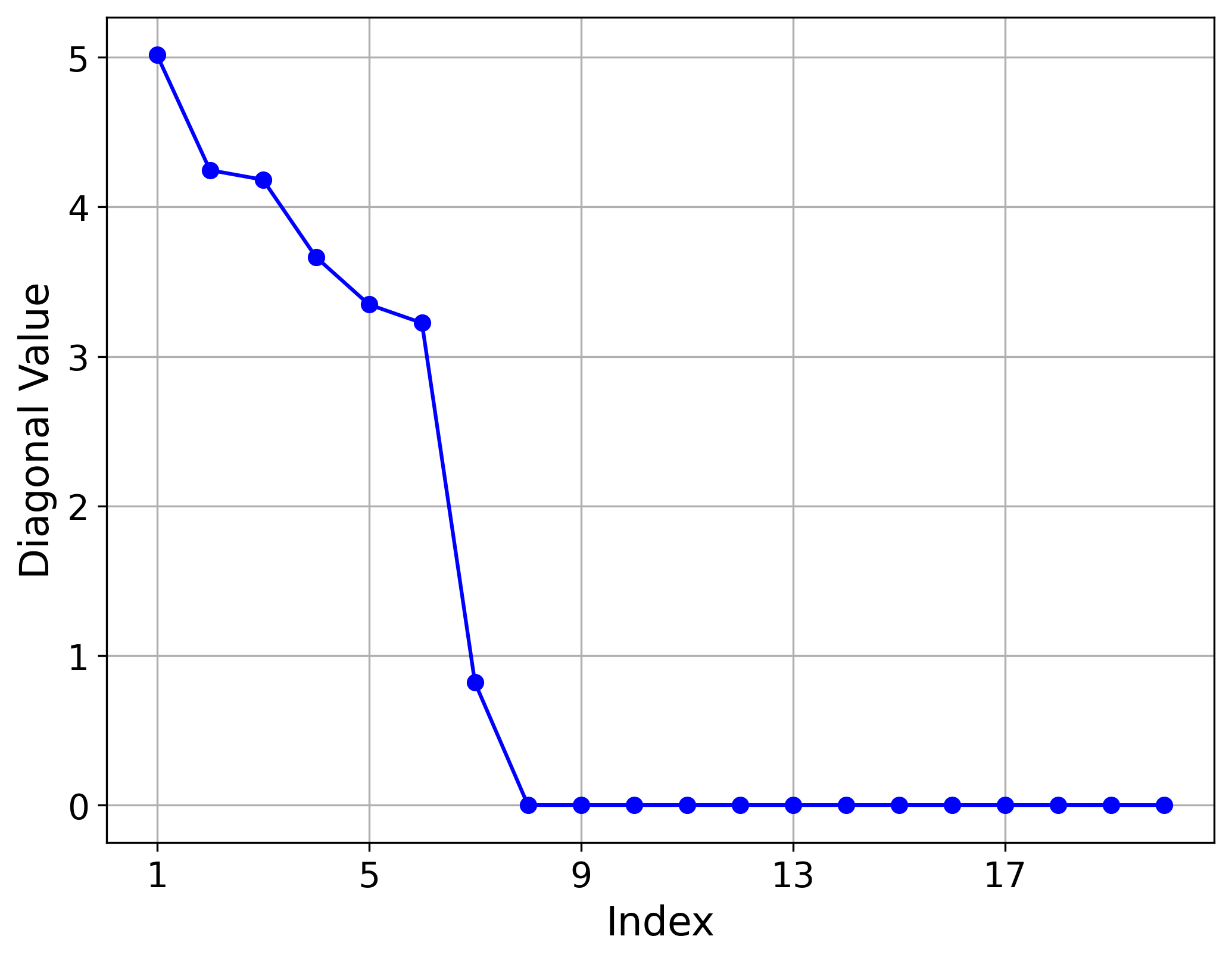
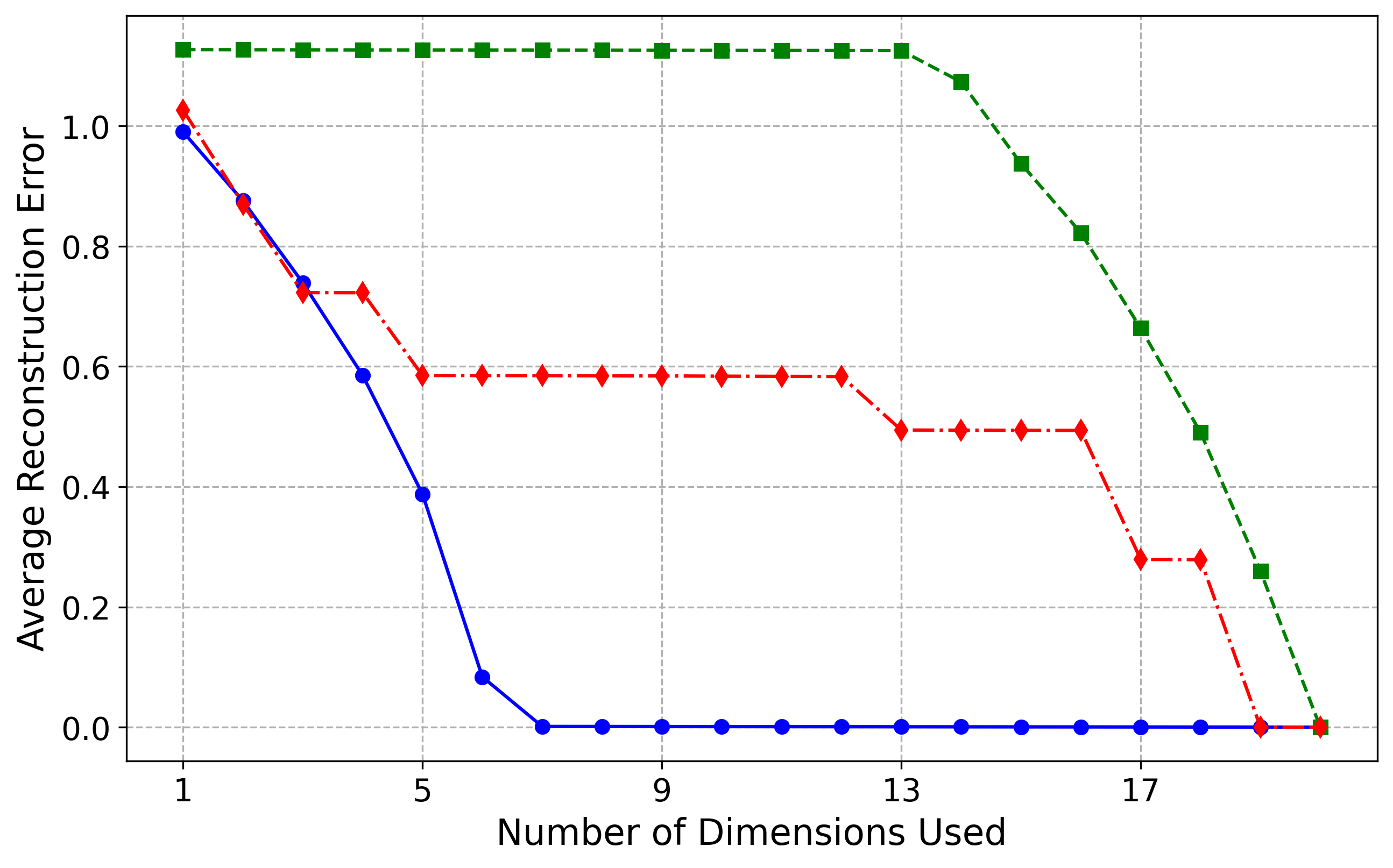
To evaluate the scalability of our approach, we applied it to higher-dimensional manifolds, specifically the Hemisphere(5,20) and Sinusoid(5,20) datasets. The figures below show, for each dataset:
- The learned variance for each latent dimension, highlighting the importance of each dimension in representing the manifold.
- The reconstruction error as a function of the number of latent dimensions used, comparing three different orders in which dimensions are added.
These three ordering strategies, shown in distinct colors, reflect different approaches to incorporating latent dimensions based on their variance:
- Blue line (circular markers): Adds dimensions in order of decreasing variance, prioritizing the most informative dimensions first.
- Green line (square markers): Adds dimensions in order of increasing variance, starting with the least significant dimensions.
- Red line (diamond markers): Adds dimensions in a random order to evaluate performance without prioritization.
This setup allows us to investigate the performance of the RAE.
Hemisphere (5,20) Results
Sinusoid (5,20) Results
Discussion of Results
For the Hemisphere(5,20) dataset, the model identified five non-vanishing variances, perfectly capturing the intrinsic dimension of the manifold. This is reflected in the blue reconstruction curve, where the first five latent dimensions, corresponding to the largest variances, are sufficient to reduce the reconstruction error almost to zero. In contrast, the green curve illustrates that the remaining ambient dimensions do not encode useful information about the manifold. The red curve demonstrates improvement only when an important latent dimension is included.
For the more challenging Sinusoid(5,20) dataset, our method still performs very well, though not as perfectly as for the Hemisphere dataset. The first six most important latent dimensions explain approximately \(97\%\) of the variance, increasing to over \(99\%\) with the seventh dimension. This is reflected in the blue reconstruction curve, where the first six latent dimensions reduce the reconstruction error to near zero, and the addition of the seventh dimension brings the error effectively to zero. The slight discrepancy between our results and the ground truth likely arises from increased optimization difficulty, as the normalizing flow must learn a more intricate distribution while maintaining approximate isometry. We believe that with deeper architectures and more careful tuning of the optimization loss, the model will converge to the correct intrinsic dimensionality of five. Currently, it predicts six dimensions at a variance threshold of \(\epsilon = 0.05\) and seven at \(\epsilon = 0.01\), slightly overestimating due to the manifold's complexity.
Manifold Mappings
To improve the stability and accuracy of learned manifold mappings, we adapted the standard normalizing flow (NF) training with two main modifications:
- Anisotropic Base Distribution: We parameterize the diagonal elements of the covariance matrix, introducing anisotropy in the base distribution.
- Isometry Regularization: Regularizing the flow to be approximately isometric, ensuring stable and interpretable mappings.
We compared our method against three baselines:
- Normalizing Flow (NF): Uses an isotropic Gaussian base distribution with no isometry regularization.
- Anisotropic Normalizing Flow: Applies the same anisotropic base distribution as our method but without isometry regularization.
- Isometric Normalizing Flow: Uses an isotropic Gaussian base distribution with (\ell^2)-isometry regularization.
Experiments were conducted on three datasets—Single Banana, Squeezed Single Banana, and River—using two metrics:
- Geodesic Error: Average deviation from ground truth geodesics.
- Variation Error: Stability under small perturbations.
Results Summary
Our method consistently outperformed all baselines, achieving lower geodesic and variation errors across all datasets, as shown in the table below.

Table: Comparison of geodesic and variation errors across datasets, highlighting our method’s superior accuracy and stability.
Visual Comparison of Geodesics
The figure below compares geodesics generated by different methods on the River dataset. Our method yields the most stable and accurate geodesics, consistent with the quantitative results.
