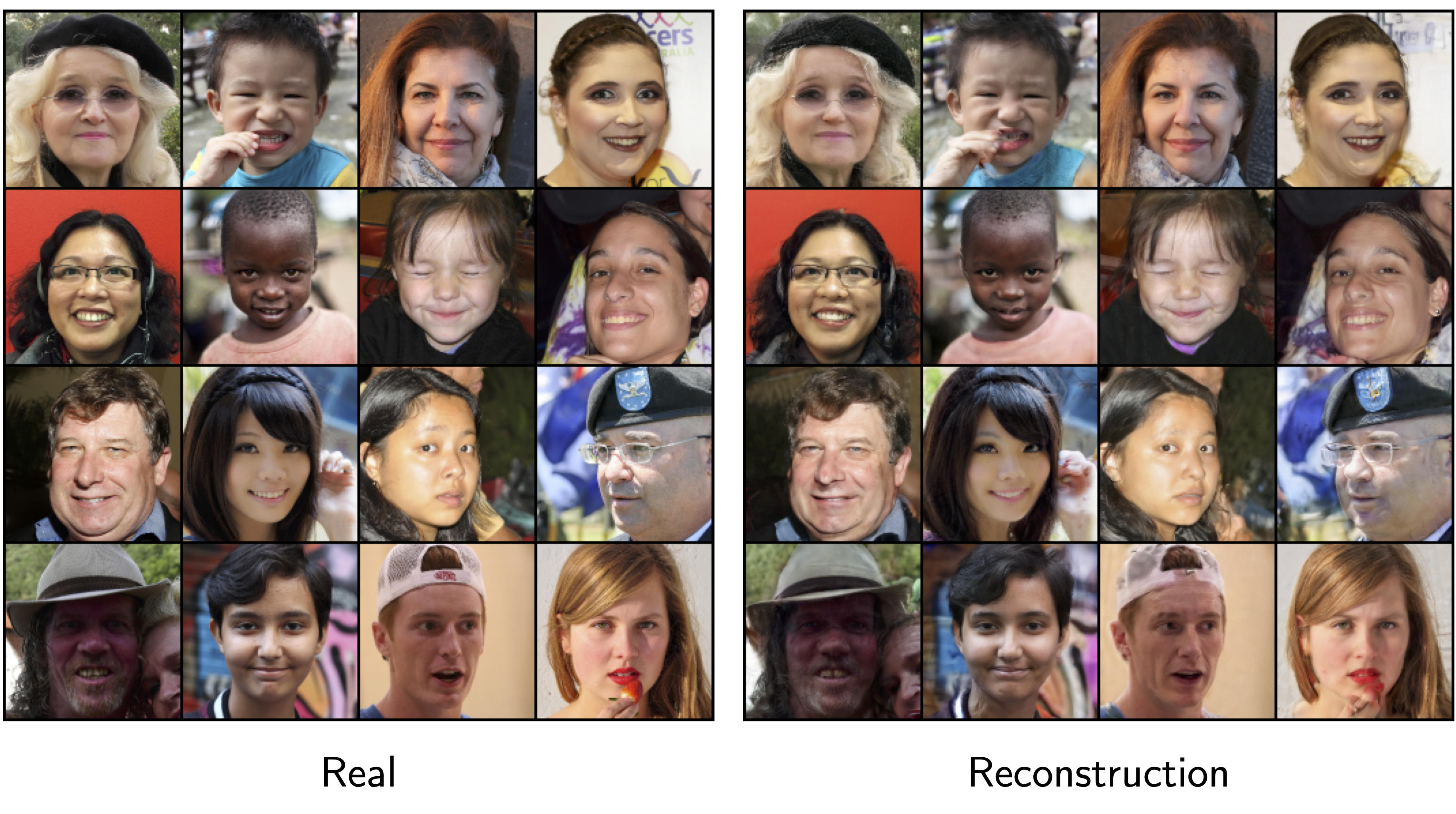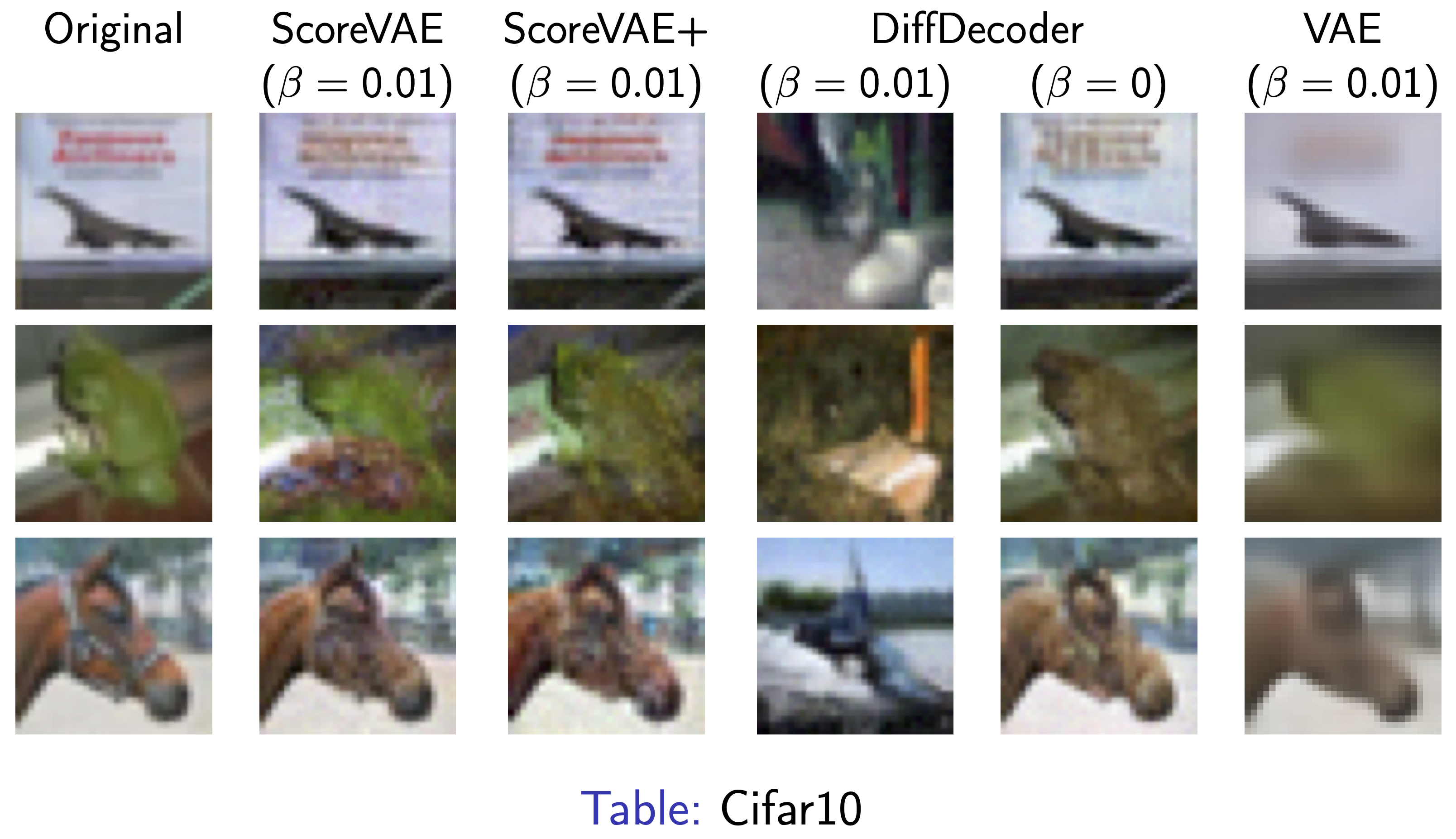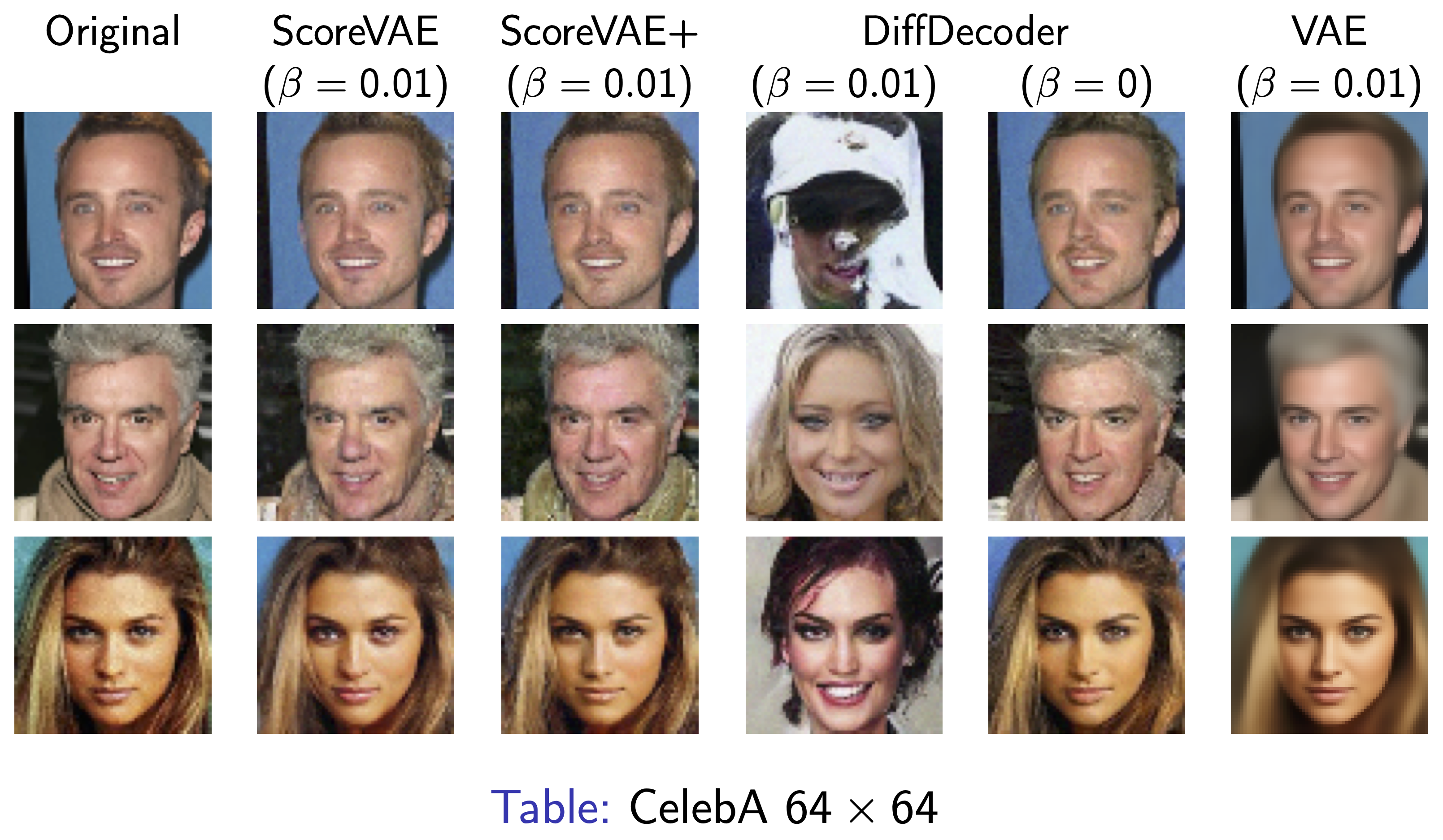
Overview
In this paper, we introduce ScoreVAE, a novel approach that advances the Variational Autoencoder (VAE) framework by addressing fundamental limitations of conventional VAEs. Traditional VAEs model the reconstruction distribution \( p(\mathbf{x} | \mathbf{z}) \) as a Gaussian, which often leads to overly smoothed and blurry reconstructions. This limitation arises because the Gaussian assumption fails to capture the complexity and multimodality of real-world data distributions, making it difficult for the model to accurately represent intricate details and sharp features. ScoreVAE addresses this issue by combining a diffusion-time dependent encoder and an unconditional diffusion model. By employing Bayes' rule for score functions, we analytically derive a robust and flexible model for reconstruction distribution \( p(\mathbf{x} | \mathbf{z}) \). Our approach bypasses the unrealistic Gaussian assumption, resulting in significantly improved image reconstruction quality.
The ScoreVAE framework also simplifies the training dynamics by decoupling the training of the diffusion model and the encoder. This decoupling enables the use of powerful pre-trained diffusion models that can be readily updated or swapped without retraining the entire system. By separating the prior (diffusion model) from the encoder, ScoreVAE achieves higher fidelity reconstructions compared to traditional VAEs and diffusion decoders. Our experiments on the CIFAR10 and CelebA datasets demonstrate ScoreVAE’s superiority in producing sharper images and reducing reconstruction error. These results underscore the practical advantages of ScoreVAE in handling complex, high-dimensional data, and highlight its potential for improved representation learning and controllable generative modeling.
Experimental Results


Derivation of the Training Objective
ELBO in Variational Autoencoders
In the Variational Autoencoder (VAE) framework, maximizing the exact log-likelihood \( \ln p_\theta(\mathbf{x}) \) is often infeasible. Instead, we optimize a tractable lower bound known as the Evidence Lower Bound (ELBO), which approximates this objective. However, a common modification introduces a hyperparameter \( \beta \), leading to the \(\beta\)-ELBO objective: \[ \text{ELBO}(\theta, \phi; \beta) = \mathbb{E}_{q_\phi(\mathbf{z} \mid \mathbf{x})} \left[ \ln p_\theta(\mathbf{x} \mid \mathbf{z}) \right] - \beta \, D_{\text{KL}} \left( q_\phi(\mathbf{z} \mid \mathbf{x}) \, \| \, p(\mathbf{z}) \right), \] where: - \( \mathbf{x} \) is the data sample, - \( \mathbf{z} \) represents the latent variable, - \( q_\phi(\mathbf{z} \mid \mathbf{x}) \) is the approximate posterior distribution (encoder), - \( p_\theta(\mathbf{x} \mid \mathbf{z}) \) is the reconstruction distribution (decoder), - \( p(\mathbf{z}) \) is the prior over the latent space, - \( \beta \in (0, 1) \) controls the weight of the KL divergence term, balancing regularization and reconstruction. This modified \(\beta\)-VAE objective is motivated by issues with the standard ELBO, where the KL penalty term can lead to over-regularization and poor convergence. By introducing \( \beta \), we can alleviate these issues, effectively adjusting the trade-off between the reconstruction term and the latent regularization.
Modeling \( p_\theta(\mathbf{x}_0 \mid \mathbf{z}) \) with a Diffusion Model
We propose to model \( p_\theta(\mathbf{x}_0 \mid \mathbf{z}) \) using a conditional diffusion model \(s_\theta(\mathbf{x}_t, \mathbf{z}, t)\) within the continuous-time score-based generative modeling framework. The log-likelihood can be lower-bounded as follows: \[ \ln p_\theta(\mathbf{x}_0 \mid \mathbf{z}) \geq C - \frac{1}{2} \int_0^T g(t)^2 \, \mathbb{E}_{p_{0t}(\mathbf{x}_t \mid \mathbf{x}_0)} \left[ \left\| s_\theta(\mathbf{x}_t, \mathbf{z}, t) - \nabla_{\mathbf{x}_t} \ln p_{0t}(\mathbf{x}_t \mid \mathbf{x}_0) \right\|^2 \right] \, \mathrm{d}t, \] where: \( \mathbf{x}_t \) is the diffused data at time \( t \), \( p_{0t}(\mathbf{x}_t \mid \mathbf{x}_0) \) is the forward diffusion process from \( \mathbf{x}_0 \) to \( \mathbf{x}_t \), \( s_\theta(\mathbf{x}_t, \mathbf{z}, t) \) is the conditional score function approximating \( \nabla_{\mathbf{x}_t} \ln p_{0t}(\mathbf{x}_t \mid \mathbf{z}) \), \( g(t) \) is the diffusion coefficient, \( C \) is a constant independent of \( \theta \).
Note that training the conditional diffusion model to minimize the conditional denoising score-matching objective (right part of the RHS of the inequality) maximizes a lower bound on the reconstruction loglikelihood. Moreover, it has been shown by Batzolis et al. (2021) that the minimizer \( s_\theta^*(\mathbf{x}_t, \mathbf{z}, t) \) of the conditional denoising score-matching objective is a consistent estimator of the conditional score \( \nabla_{\mathbf{x}_t} \ln p_t(\mathbf{x}_t \mid \mathbf{z}) \).
Decomposing the Conditional Score Function
Using Bayes' rule for score functions, we decompose the conditional score \(\nabla_{\mathbf{x}_t} \ln p_{t}(\mathbf{x}_t \mid \mathbf{z})\) into an unconditional score and a latent correction score as follows: \[ \nabla_{\mathbf{x}_t} \ln p_{t}(\mathbf{x}_t \mid \mathbf{z}) = \nabla_{\mathbf{x}_t} \ln p_{t}(\mathbf{x}_t) + \nabla_{\mathbf{x}_t} \ln p(\mathbf{z} \mid \mathbf{x}_t). \]
Approximating the Unconditional Score with a Pre-trained Model
To approximate the unconditional score \( \nabla_{\mathbf{x}_t} \ln p_{t}(\mathbf{x}_t) \), we use a pre-trained unconditional diffusion model \( s_p(\mathbf{x}_t, t) \): \[ s_p(\mathbf{x}_t, t) \approx \nabla_{\mathbf{x}_t} \ln p_{t}(\mathbf{x}_t). \]
Modeling the Latent Correction Score with a Time-Dependent Encoder
Direct computation of \( \nabla_{\mathbf{x}_t} \ln p(\mathbf{z} \mid \mathbf{x}_t) \) is intractable. We approximate it by assuming: \[ p(\mathbf{z} \mid \mathbf{x}_t) \approx q_\phi(\mathbf{z} \mid \mathbf{x}_t), \] where \( q_\phi(\mathbf{z} \mid \mathbf{x}_t) \) is a Gaussian distribution parameterized by a time-dependent encoder \( e_\phi(\mathbf{x}_t, t) \): \[ q_\phi(\mathbf{z} \mid \mathbf{x}_t) = \mathcal{N} \left( \mathbf{z}; \mu_\phi(\mathbf{x}_t, t), \Sigma_\phi(\mathbf{x}_t, t) \right). \] The score \( \nabla_{\mathbf{x}_t} \ln q_\phi(\mathbf{z} \mid \mathbf{x}_t) \) can be computed analytically due to the Gaussian assumption.
Formulating the Combined Score Function
Our approximation of the conditional score function is then: \[ s_\theta(\mathbf{x}_t, \mathbf{z}, t) = s_p(\mathbf{x}_t, t) + \nabla_{\mathbf{x}_t} \ln q_\phi(\mathbf{z} \mid \mathbf{x}_t). \]
Deriving the Training Objective
Substituting this into the lower bound of \( \ln p_\theta(\mathbf{x}_0 \mid \mathbf{z}) \), we get: \[ \ln p_\theta(\mathbf{x}_0 \mid \mathbf{z}) \geq C - \frac{1}{2} \int_0^T g(t)^2 \, \mathbb{E}_{p_{0t}(\mathbf{x}_t \mid \mathbf{x}_0)} \left[ \left\| s_p(\mathbf{x}_t, t) + \nabla_{\mathbf{x}_t} \ln q_\phi(\mathbf{z} \mid \mathbf{x}_t) - \nabla_{\mathbf{x}_t} \ln p_{0t}(\mathbf{x}_t \mid \mathbf{x}_0) \right\|^2 \right] \, \mathrm{d}t. \] Since \( s_p(\mathbf{x}_t, t) \) is pre-trained and fixed, the learnable parameters reside in the encoder \( e_\phi \).
Final Training Objective
Combining the lower the lower bound of \( \ln p_\theta(\mathbf{x}_0 \mid \mathbf{z}) \) with the KL-penalty term, we get the following training objective which is a lower bound of the \(\beta\)-ELBO objective: \[ \mathcal{L}(\phi) = \mathbb{E}_{\mathbf{x}_0 \sim p(\mathbf{x}_0)} \left[ \frac{1}{2} \, \mathbb{E}_{\substack{t \sim \mathcal{U}(0, T) \\ \mathbf{x}_t \sim p_{0t}(\mathbf{x}_t \mid \mathbf{x}_0) \\ \mathbf{z} \sim q_\phi(\mathbf{z} \mid \mathbf{x}_0)}} \left[ g(t)^2 \left\| \nabla_{\mathbf{x}_t} \ln p_{0t}(\mathbf{x}_t \mid \mathbf{x}_0) - s_p(\mathbf{x}_t, t) - \nabla_{\mathbf{x}_t} \ln q_\phi(\mathbf{z} \mid \mathbf{x}_t) \right\|^2 \right] + \beta\, D_{\text{KL}} \left( q_\phi(\mathbf{z} \mid \mathbf{x}_0) \, \| \, p(\mathbf{z}) \right) \right]. \] where: \( \mathbf{x}_0 \sim p(\mathbf{x}_0) \) is sampled from the data distribution, \( \mathbf{z} \sim q_\phi(\mathbf{z} \mid \mathbf{x}_0) \) is sampled from the encoder's approximate posterior at \( t = 0 \), \( t \sim \mathcal{U}(0, T) \) is sampled uniformly over the diffusion time, \( \mathbf{x}_t \sim p_{0t}(\mathbf{x}_t \mid \mathbf{x}_0) \) is obtained by diffusing \( \mathbf{x}_0 \) forward to time \( t \). This objective encourages the encoder to produce latent representations that are informative about \( \mathbf{x}_0 \) while maintaining closeness to the prior \( p(\mathbf{z}) \).
